Source repo for Colab bootstrap and helper downloads: https://gitlab.com/cam-ml/tutorials/-/tree/main/notebooks/05-generative

Diffusion Fundamentals: DDPM, Score-Based Models, NCSN, and DDIM¶

This notebook is the conceptual warm-up on diffusion models.

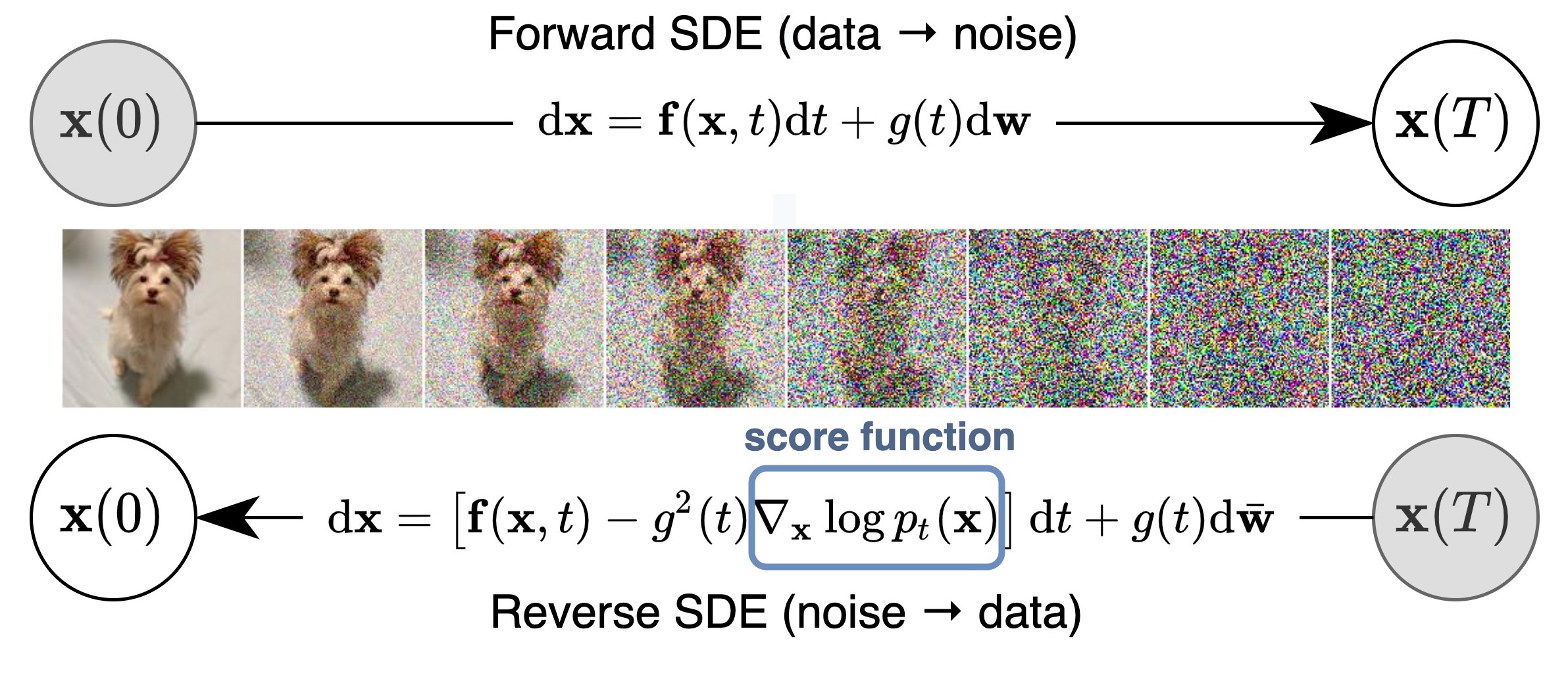
Score-SDE schematic from the official repository

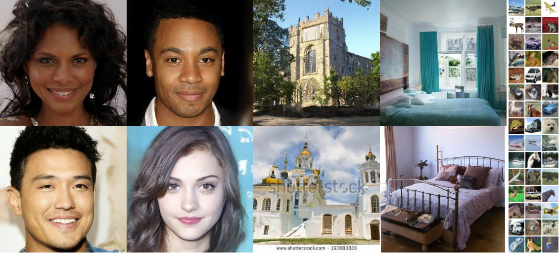
Source: Yang Song et al., Score-Based Generative Modeling through Stochastic Differential Equations (ICLR 2021), official score_sde_pytorch repository README figure assets/schematic.jpg: https://github.com/yang-song/score_sde_pytorch

DDPM samples from the official repository

Source: Jonathan Ho, Ajay Jain, and Pieter Abbeel, Denoising Diffusion Probabilistic Models (2020), official diffusion repository README figure resources/samples.png: https://github.com/hojonathanho/diffusion

Aims¶

build physical intuition from energy landscapes, stochastic motion, and Langevin dynamics,
connect that intuition to the forward-noising / reverse-denoising recipe,
compare three concrete model families on the same toy dataset: NCSN / score-based models, DDPM, and DDIM,
prepare for the crystal notebooks by separating “representation questions” from “diffusion questions”.

Learning outcomes¶

By the end you should be able to:

explain what the score is and why Langevin dynamics matters,
describe what NCSN, DDPM, and DDIM learn and how they sample,
say clearly what DDPM and DDIM share and what changes between them,
connect the toy examples here to the crystal-generation workflow later in Day 5.

Key references for this notebook¶

This notebook is pedagogical, but the model families and notation come from a small set of canonical papers:

Ho, Jain, and Abbeel, Denoising Diffusion Probabilistic Models (DDPM): https://arxiv.org/abs/2006.11239
Song and Ermon, Generative Modeling by Estimating Gradients of the Data Distribution (NCSN): https://arxiv.org/abs/1907.05600
Song et al., Score-Based Generative Modeling through Stochastic Differential Equations: https://arxiv.org/abs/2011.13456
Song, Meng, and Ermon, Denoising Diffusion Implicit Models (DDIM): https://arxiv.org/abs/2010.02502

The code here is intentionally small and CPU-friendly, so it illustrates the core ideas rather than reproducing the full training setups from the papers.

Table of Contents¶

Key references for this notebook
Part 1: Energy landscapes, drift, and stochastic motion
Part 1A: Numerical integration as repeated local updates
Part 1B: Brownian motion and Ornstein--Uhlenbeck intuition
Temperature intuition: particles in a double-well landscape
Part 2: Langevin dynamics and equilibrium sampling
Transition: from Langevin intuition to diffusion models
Part 3: A single toy dataset for all three model families
Forward corruption preview
Part 3A: NCSN and score-based models
Part 3B: DDPM
Part 3C: DDIM
Part 3D: What actually differs?
Part 4: Bridge to crystals

If you already know the ODE/SDE warm-up, you can jump straight to Part 3 for the concrete model comparison.

# @title
from pathlib import Path
import os
import subprocess
import sys
from typing import Optional

import numpy as np
from matplotlib import pyplot as plt
from matplotlib.axes._axes import Axes
import seaborn as sns
import torch
import torch.distributions as D
from torch.func import vmap, jacrev
from tqdm import tqdm

try:
    import ipywidgets as widgets
except Exception:
    widgets = None

try:
    import google.colab  # type: ignore
    IN_COLAB = True
except Exception:
    IN_COLAB = False

from IPython.display import display

device = torch.device('cuda' if torch.cuda.is_available() else 'cpu')

DAY5_SOURCE_REPO_URL = "https://gitlab.com/cam-ml/tutorials.git"
DAY5_SOURCE_REPO_BRANCH = "main"
DAY5_COLAB_CLONE_CANDIDATES = [
    Path("/content/tutorials"),
    Path("/content/cam_ml_tutorials"),
    Path("/content/camml-tutorials"),
]


def _running_in_colab():
    try:
        import google.colab  # type: ignore
        return True
    except Exception:
        return False


def _unique_paths(paths):
    unique = []
    seen = set()
    for path in paths:
        path = Path(path)
        key = str(path)
        if key not in seen:
            seen.add(key)
            unique.append(path)
    return unique


def _iter_day5_search_roots():
    cwd = Path.cwd().resolve()
    roots = [cwd, *cwd.parents]
    for clone_dir in DAY5_COLAB_CLONE_CANDIDATES:
        roots.extend([clone_dir, clone_dir / "notebooks" / "05-generative"])
    return _unique_paths(roots)


def _register_day5_notebook_root(notebook_root: Path):
    notebook_root = notebook_root.resolve()
    if str(notebook_root) not in sys.path:
        sys.path.insert(0, str(notebook_root))
    try:
        os.chdir(notebook_root)
    except OSError:
        pass
    return notebook_root


def ensure_day5_helpers_on_path():
    for candidate in _iter_day5_search_roots():
        for notebook_root in (candidate, candidate / "notebooks" / "05-generative"):
            helper_dir = notebook_root / "gen_helpers"
            if helper_dir.exists():
                return _register_day5_notebook_root(notebook_root)

    if _running_in_colab():
        for clone_dir in DAY5_COLAB_CLONE_CANDIDATES:
            notebook_root = clone_dir / "notebooks" / "05-generative"
            if notebook_root.exists():
                return _register_day5_notebook_root(notebook_root)

        for clone_dir in DAY5_COLAB_CLONE_CANDIDATES:
            if clone_dir.exists():
                continue
            clone_dir.parent.mkdir(parents=True, exist_ok=True)
            print(
                "Cloning the Day 5 tutorial repo from "
                f"{DAY5_SOURCE_REPO_URL} into {clone_dir} so notebook helper modules are available..."
            )
            subprocess.run(
                [
                    "git",
                    "clone",
                    "--depth",
                    "1",
                    "--branch",
                    DAY5_SOURCE_REPO_BRANCH,
                    DAY5_SOURCE_REPO_URL,
                    str(clone_dir),
                ],
                check=True,
            )
            notebook_root = clone_dir / "notebooks" / "05-generative"
            if notebook_root.exists():
                return _register_day5_notebook_root(notebook_root)

        raise FileNotFoundError(
            "Could not find or clone notebooks/05-generative inside /content for this Colab session."
        )

    raise FileNotFoundError(
        "Could not locate notebooks/05-generative/gen_helpers. If you are in Colab, rerun this cell so the repo can be cloned automatically."
    )

GEN_HELPERS_ROOT = ensure_day5_helpers_on_path()

from gen_helpers.fundamentals_helpers import bind_widget_state, figure_to_png_bytes

Part 1: Energy landscapes, drift, and stochastic motion¶

Let us make precise the central objects of study: ordinary differential equations (ODEs) and stochastic differential equations (SDEs).

In this notebook, you can interpret the time-dependent score field

u:\mathbb{R}^d\times [0,1]\to \mathbb{R}^d,\qquad (x,t)\mapsto u_t(x)

(1)

as an effective velocity field in configuration space. In chemistry language, this is analogous to saying:

the system is currently at configuration $x$ ,
at time $t$ ,
and the local geometry of the landscape tells us which way the configuration wants to move.

An ODE is then

dX_t = u_t(X_t)\,dt, \qquad X_0=x_0.

(2)

This is the deterministic case: once the initial condition is fixed, the trajectory is fixed. Conceptually, this is like continuous-time relaxation or steepest-descent-style motion on an energy landscape.

An SDE is

dX_t = u_t(X_t)\,dt + \sigma_t\, dW_t,\qquad X_0=x_0,

(3)

which adds a stochastic term driven by Brownian motion $(W_t)_{0\le t\le 1}$ . Here:

$u_t(X_t)$ is the drift,
$\sigma_t$ is the diffusion coefficient,
and the stochastic term plays the role of thermal agitation / random kicks.

So the mental model is:

ODE = deterministic relaxation
SDE = deterministic relaxation + thermal/random fluctuations

That same language will become very useful later, because diffusion models can be viewed as learning how to reverse a noising process in exactly this SDE/ODE framework.

Translation guide: math language $\leftrightarrow$ chemistry / materials language¶

Math / generative modeling	Chemistry / materials intuition
state $x$	configuration, coordinate, structure descriptor
drift $u_t(x)$	deterministic velocity / force-induced motion
diffusion coefficient $\sigma_t$	noise strength, temperature-like stochasticity
Brownian motion	free diffusion
OU process	diffusion in a harmonic basin
$\nabla \log p(x)$ (score)	force-like field toward high-probability / low-energy regions
Langevin dynamics	noisy force-driven sampling
stationary distribution	equilibrium distribution

You do not need to think of these as separate formulations. The same equations appear in both.

Note. You can indeed view an ODE as the zero-noise limit of an SDE. We will still treat them separately here, because it keeps the simulation schemes and the physical intuition cleaner.

# Shared simulator utilities for the exercises below.
def make_simulator(step_fn):
    return {"step": step_fn}


@torch.no_grad()
def simulate(simulator, x: torch.Tensor, ts: torch.Tensor):
    for t_idx in range(len(ts) - 1):
        t = ts[t_idx]
        h = ts[t_idx + 1] - ts[t_idx]
        x = simulator["step"](x, t, h)
    return x


@torch.no_grad()
def simulate_with_trajectory(simulator, x: torch.Tensor, ts: torch.Tensor):
    xs = [x.clone()]
    for t_idx in tqdm(range(len(ts) - 1)):
        t = ts[t_idx]
        h = ts[t_idx + 1] - ts[t_idx]
        x = simulator["step"](x, t, h)
        xs.append(x.clone())
    return torch.stack(xs, dim=1)


def plot_trajectories_1d(
    x0: torch.Tensor,
    simulator,
    timesteps: torch.Tensor,
    ax: Optional[Axes] = None,
    show_hist: bool = False,
    decouple_hist_axis: bool = False,
):
    if ax is None:
        ax = plt.gca()
    trajectories = simulate_with_trajectory(simulator, x0, timesteps)

    line_color = sns.color_palette("crest", 1)[0]
    hist_color = sns.color_palette("flare", 1)[0]
    label_size = 12
    tick_size = 10

    timesteps_cpu = timesteps.detach().cpu().numpy()
    for trajectory_idx in range(trajectories.shape[0]):
        trajectory = trajectories[trajectory_idx, :, 0].detach().cpu().numpy()
        sns.lineplot(
            x=timesteps_cpu,
            y=trajectory,
            ax=ax,
            color=line_color,
            alpha=0.45,
            linewidth=1.1,
            legend=False,
        )

    ax.set_xlabel(r"time ($t$)", fontsize=label_size)
    ax.set_ylabel(r"$X_t$", fontsize=label_size)
    ax.tick_params(axis="both", labelsize=tick_size)
    ax.grid(alpha=0.2, linewidth=0.6)

    if show_hist:
        terminal_points = trajectories[:, -1, 0].detach().cpu().numpy()
        data_range = float(terminal_points.max() - terminal_points.min()) if terminal_points.size else 1.0
        binwidth = max(data_range / 25.0, 0.05)

        from mpl_toolkits.axes_grid1 import make_axes_locatable

        divider = make_axes_locatable(ax)
        sharey = None if decouple_hist_axis else ax
        hist_ax = divider.append_axes("right", size="22%", pad=0.45, sharey=sharey)
        sns.histplot(
            y=terminal_points,
            ax=hist_ax,
            binwidth=binwidth,
            color=hist_color,
            alpha=0.7,
            edgecolor="white",
            linewidth=0.5,
        )
        hist_ax.set_xlabel("count", fontsize=label_size)
        hist_ax.set_ylabel("")
        hist_ax.tick_params(axis="both", labelsize=tick_size)
        if decouple_hist_axis:
            hist_ax.tick_params(axis="y", left=True, labelleft=True)
        else:
            hist_ax.tick_params(axis="y", left=False, labelleft=False)
        hist_ax.grid(axis="x", alpha=0.2, linewidth=0.6)

    fig = ax.figure
    if fig is not None:
        title = ax.get_title()
        if title:
            title_size = ax.title.get_fontsize()
            ax.set_title("")

            axes = [ax]
            if show_hist:
                axes.append(hist_ax)

            fig.canvas.draw()
            bboxes = [a.get_position() for a in axes]

            left = min(b.x0 for b in bboxes)
            right = max(b.x1 for b in bboxes)
            top = max(b.y1 for b in bboxes)

            x_center = 0.5 * (left + right)
            y = top + 0.005

            fig.text(
                x_center,
                y,
                title,
                ha="center",
                va="bottom",
                fontsize=title_size,
            )

Part 1A: Numerical integration as repeated local updates¶

In practice, we almost never solve these equations analytically. Instead, we integrate them numerically, exactly as you would do for equations of motion in simulation.

If we think of $X_t$ as the current configuration, then an ODE says:

update the configuration according to the local drift field.

For the ODE

dX_t = u_t(X_t)\,dt,

(4)

the explicit Euler step is

X_{t+h} = X_t + h\,u_t(X_t),

(5)

where $h=\Delta t$ is the step size.

For the SDE

dX_t = u_t(X_t)\,dt + \sigma_t\,dW_t,

(6)

the Euler-Maruyama step is

X_{t+h} = X_t + h\,u_t(X_t) + \sigma_t \sqrt{h}\,\xi_t,

(7)

where $\xi_t\sim\mathcal{N}(0,I)$ .

This is the stochastic analogue of a basic explicit integrator: deterministic motion from the drift, plus a random increment whose scale grows like $\sqrt{h}$ . If you come from Brownian dynamics or overdamped Langevin dynamics, this form should look very familiar.

Question 1.1: Implement explicit integrators for deterministic and stochastic dynamics¶

Try first: before running the next three code cells, write down the Euler and Euler-Maruyama updates in a scratch cell or on paper.

Connect each term to the physical picture:

deterministic displacement from the drift,
a Gaussian kick for the stochastic case,
and the $\sqrt{\Delta t}$ scaling because a Wiener increment has variance $\Delta t$ .

The first code cell below defines the shared simulation loop so we can focus the exercises on the local update rules. The next two code cells are intentionally incomplete: fill the TODOs yourself, or open the hidden solutions if you want to compare against a reference implementation.

Hint: The drift should be a function that depends on the position $x_t$ and time $t$ . For normally distributed random variables, you cna use torch.randn_like()

def make_euler_maruyama_simulator(drift_coefficient, diffusion_coefficient):
    def step(xt: torch.Tensor, t: torch.Tensor, h: torch.Tensor):
        noise = diffusion_coefficient(xt, t) * torch.sqrt(h) * torch.randn_like(xt)
        return xt + drift_coefficient(xt, t) * h + noise

    return make_simulator(step)

def make_euler_simulator(drift_coefficient):
    def step(xt: torch.Tensor, t: torch.Tensor, h: torch.Tensor):
        # TODO: implement one explicit Euler step.
        raise NotImplementedError

    return make_simulator(step)

def make_euler_maruyama_simulator(drift_coefficient, diffusion_coefficient):
    def step(xt: torch.Tensor, t: torch.Tensor, h: torch.Tensor):
        # TODO: add the drift step and the stochastic kick.
        raise NotImplementedError

    return make_simulator(step)

Note. When the diffusion coefficient is zero, Euler-Maruyama reduces to ordinary Euler. In other words, the stochastic simulator collapses back to a purely deterministic integrator.

Part 1B: Brownian motion and Ornstein-Uhlenbeck intuition¶

We now build intuition for two especially important SDEs.

From a chemistry/materials viewpoint, these are good toy models for motion on simple landscapes:

Brownian motion = diffusion on a flat landscape with no restoring force,
Ornstein-Uhlenbeck (OU) = diffusion in a harmonic basin with a linear restoring force.

These two examples already contain most of the qualitative ingredients we care about later: random exploration, drift toward preferred regions, and approach to an equilibrium distribution.

Example 2.1: Brownian motion as free diffusion¶

Brownian motion is the case with no drift and constant diffusion:

dX_t = \sigma\,dW_t,\qquad X_0=0.

(8)

You can think of this as motion on a perfectly flat potential energy surface. There is no force pulling the particle anywhere in particular; it only wanders because of random kicks.

Try first: before running the Brownian-motion code, predict the trajectories qualitatively.

How should the paths look when sigma is very large? What about when sigma is close to zero?

Try first: pause and decide what the drift and diffusion should be for Brownian motion.

In physical language there is no restoring force, so the drift is zero, while the noise strength is spatially uniform.

Fill in the TODOs in the next code cell before you run it. If you get stuck, open the hidden solution.

Brownian motion satisfies

dX_t = \sigma\,dW_t.

So the drift coefficient is

b(x,t)=0,

and the diffusion coefficient is the constant field

\sigma(x,t)=\sigma.

In tensor code that means:

def make_brownian_motion(sigma: float):
    def drift_coefficient(xt: torch.Tensor, t: torch.Tensor) -> torch.Tensor:
        return torch.zeros_like(xt)

    def diffusion_coefficient(xt: torch.Tensor, t: torch.Tensor) -> torch.Tensor:
        return sigma * torch.ones_like(xt)

    return drift_coefficient, diffusion_coefficient

def make_brownian_motion(sigma: float):
    def drift_coefficient(xt: torch.Tensor, t: torch.Tensor) -> torch.Tensor:
        # TODO: Brownian motion has no deterministic drift.
        raise NotImplementedError

    def diffusion_coefficient(xt: torch.Tensor, t: torch.Tensor) -> torch.Tensor:
        # TODO: Brownian motion uses a spatially uniform noise amplitude.
        raise NotImplementedError

    return drift_coefficient, diffusion_coefficient

Now let us plot trajectories. As you inspect the figures, try to think simultaneously in two ways:

as individual paths in time, and
as an evolving ensemble of configurations.

That ensemble viewpoint is the one that later becomes central for generative modeling.

sigma = 1.0
n_traj = 500
brownian_drift, brownian_diffusion = make_brownian_motion(sigma)
simulator = make_euler_maruyama_simulator(brownian_drift, brownian_diffusion)
x0 = torch.zeros(n_traj,1).to(device) # Initial values - let's start at zero
ts = torch.linspace(0.0,5.0,500).to(device) # simulation timesteps

plt.figure(figsize=(9, 6))
ax = plt.gca()
ax.set_title(r'Trajectories of Brownian Motion with $\sigma=$' + str(sigma), fontsize=18)
ax.set_xlabel(r'time ($t$)', fontsize=18)
ax.set_ylabel(r'$x_t$', fontsize=18)
plot_trajectories_1d(x0, simulator, ts, ax, show_hist=True)
plt.show()

Question: What happens when you vary the value of sigma?

Question: Can you tell what the time-dependence of the noise is?

Example 2.2: Ornstein-Uhlenbeck as diffusion in a harmonic well¶

The OU process is

dX_t = -\theta X_t\,dt + \sigma\,dW_t,\qquad X_0=x_0.

(9)

This is one of the cleanest SDEs to interpret physically. The drift term $-\theta X_t$ is a linear restoring force that pulls the system back toward the origin, so you can view it as motion in a quadratic potential

U(x)\propto x^2.

(10)

Brownian motion wandered on a flat landscape; the OU process wanders in a basin.

Try first: predict the qualitative behavior before you run the OU-process code.

What should happen when theta is very small? What about when theta is very large?

Try first: write down the OU drift and diffusion before you inspect the next code cell.

Interpretation:

theta controls how stiff the harmonic well is,
sigma controls how strongly thermal noise kicks the system around.

Fill in the TODOs in the next code cell before you run it. If you want to check your work, open the hidden solution.

The Ornstein-Uhlenbeck process is

dX_t = -\theta X_t\,dt + \sigma\,dW_t.

So the drift coefficient is

b(x,t) = -\theta x,

and the diffusion coefficient is again spatially uniform:

\sigma(x,t)=\sigma.

That gives the implementation:

def make_ou_process(theta: float, sigma: float):
    def drift_coefficient(xt: torch.Tensor, t: torch.Tensor) -> torch.Tensor:
        return -theta * xt

    def diffusion_coefficient(xt: torch.Tensor, t: torch.Tensor) -> torch.Tensor:
        return sigma * torch.ones_like(xt)

    return drift_coefficient, diffusion_coefficient

def make_ou_process(theta: float, sigma: float):
    def drift_coefficient(xt: torch.Tensor, t: torch.Tensor) -> torch.Tensor:
        # TODO: add the linear restoring-force drift.
        raise NotImplementedError

    def diffusion_coefficient(xt: torch.Tensor, t: torch.Tensor) -> torch.Tensor:
        # TODO: keep the noise strength uniform in space.
        raise NotImplementedError

    return drift_coefficient, diffusion_coefficient

# Try comparing multiple choices side-by-side
thetas_and_sigmas = [
    (0.25, 0.0),
    (0.25, 0.5),
    (0.25, 2.0),
]
simulation_time = 10.0

num_plots = len(thetas_and_sigmas)
fig, axes = plt.subplots(2, num_plots, figsize=(10.5 * num_plots, 15))

# Top row: dynamics
n_traj = 10
for idx, (theta, sigma) in enumerate(thetas_and_sigmas):
    ou_drift, ou_diffusion = make_ou_process(theta, sigma)
    simulator = make_euler_maruyama_simulator(ou_drift, ou_diffusion)
    x0 = torch.linspace(-10.0,10.0,n_traj).view(-1,1).to(device) # Initial values - let's start at zero
    ts = torch.linspace(0.0,simulation_time,1000).to(device) # simulation timesteps

    ax = axes[0,idx]
    ax.set_title(fr'Trajectories of OU Process with $\sigma = {sigma}, \theta = {theta}$', fontsize=15)
    plot_trajectories_1d(x0, simulator, ts, ax, show_hist=False)

# Bottom row: distribution
n_traj = 500
for idx, (theta, sigma) in enumerate(thetas_and_sigmas):
    ou_drift, ou_diffusion = make_ou_process(theta, sigma)
    simulator = make_euler_maruyama_simulator(ou_drift, ou_diffusion)
    x0 = torch.linspace(-10.0,10.0,n_traj).view(-1,1).to(device) # Initial values - let's start at zero
    ts = torch.linspace(0.0,simulation_time,1000).to(device) # simulation timesteps

    ax = axes[1,idx]
    ax.set_title(fr'Trajectories of OU Process with $\sigma = {sigma}, \theta = {theta}$', fontsize=15)
    ax = plot_trajectories_1d(x0, simulator, ts, ax, show_hist=True, decouple_hist_axis=True)
plt.show()

Your job: What do you notice about the long-time behavior? Are the trajectories converging to a single point, or to a distribution?

Think about:

“When ( $\theta$ or $\sigma$ ) goes (up or down), we see ...”

Hint. Keep an eye on the ratio

D \triangleq \frac{\sigma^2}{2\theta}.

(11)

From a statistical mechanics perspective, this ratio plays the role of the equilibrium variance of the stationary Gaussian.

Your answer:

# Let's compare various OU processes!
sigmas = [1.0, 2.0, 10.0]
ds = [0.25, 1.0, 4.0] # sigma**2 / 2t
simulation_time = 15.0
n_traj = 100

fig, axes = plt.subplots(len(ds), len(sigmas), figsize=(8 * len(sigmas), 8 * len(ds)))
axes = axes.reshape((len(ds), len(sigmas)))
for d_idx, d in enumerate(ds):
    for s_idx, sigma in enumerate(sigmas):
        theta = sigma**2 / 2 / d
        ou_drift, ou_diffusion = make_ou_process(theta, sigma)
        simulator = make_euler_maruyama_simulator(ou_drift, ou_diffusion)
        x0 = torch.linspace(-20.0,20.0,n_traj).view(-1,1).to(device)
        time_scale = sigma**2
        ts = torch.linspace(0.0,simulation_time / time_scale,1000).to(device) # simulation timesteps
        ax = axes[d_idx, s_idx]
        ax.set_title(f'OU Trajectories with Sigma={sigma}, Theta={theta}, D={d}')
        plot_trajectories_1d(x0=x0, simulator=simulator, timesteps=ts, ax=ax, show_hist=True, decouple_hist_axis=True)
        ax.set_xlabel(r'$t$')
        ax.set_ylabel(r'X_t')
plt.show()

Question: What conclusion can we draw from the figure above? One qualitative sentence is fine. We will revisit this in Section 3.2.

Temperature intuition: particles in a double-well landscape¶

Before we jump to learned diffusion models, it helps to watch particles move on a simple energy surface.

We use an overdamped Langevin update in a double-well potential

U(x, y) = \tfrac{1}{4}(x^2 - 1.5)^2 + 0.7 y^2,

(12)

so there are two preferred basins, one on the left and one on the right.

The update is

X_{k+1} = X_k - \nabla U(X_k)\,\Delta t + \sqrt{2T\,\Delta t}\,\xi_k,

(13)

where $T$ plays the role of a temperature-like noise strength.

What to notice¶

Low temperature means the particle mostly rattles inside one basin.
Higher temperature means barrier-crossing becomes more common.
This is the same drift-plus-noise picture we will later reuse in reverse-time diffusion sampling.

import math

def double_well_potential(xy: torch.Tensor) -> torch.Tensor:
    x = xy[..., 0]
    y = xy[..., 1]
    return 0.25 * (x ** 2 - 1.5) ** 2 + 0.7 * y ** 2


def double_well_grad(xy: torch.Tensor) -> torch.Tensor:
    x = xy[..., 0]
    y = xy[..., 1]
    dUx = x * (x ** 2 - 1.5)
    dUy = 1.4 * y
    return torch.stack([dUx, dUy], dim=-1)


@torch.no_grad()
def simulate_double_well(
    temperature: float = 0.10,
    n_particles: int = 24,
    n_steps: int = 180,
    dt: float = 0.03,
    seed: int = 0,
):
    torch.manual_seed(seed)
    start = torch.randn(n_particles, 2, device=device) * 0.18
    start[:, 0] -= 1.1
    x = start.clone()
    traj = [x.detach().cpu()]
    for _ in range(n_steps):
        drift = -double_well_grad(x)
        noise = math.sqrt(2.0 * temperature * dt) * torch.randn_like(x)
        x = x + dt * drift + noise
        traj.append(x.detach().cpu())
    return torch.stack(traj, dim=0)


def build_double_well_demo_figure(
    temperature: float = 0.10,
    n_particles: int = 24,
    n_steps: int = 180,
    dt: float = 0.03,
    seed: int = 0,
):
    traj = simulate_double_well(
        temperature=temperature,
        n_particles=n_particles,
        n_steps=n_steps,
        dt=dt,
        seed=seed,
    )
    grid_x = torch.linspace(-2.2, 2.2, 180)
    grid_y = torch.linspace(-1.8, 1.8, 180)
    xx, yy = torch.meshgrid(grid_x, grid_y, indexing='xy')
    grid = torch.stack([xx, yy], dim=-1)
    energy = double_well_potential(grid).numpy()

    fig, axes = plt.subplots(1, 2, figsize=(12, 4.8))

    axes[0].contourf(grid_x.numpy(), grid_y.numpy(), energy, levels=30, cmap='cividis')
    for idx in range(min(n_particles, traj.shape[1])):
        path = traj[:, idx, :]
        axes[0].plot(path[:, 0], path[:, 1], alpha=0.45, linewidth=1.0)
    axes[0].scatter(traj[0, :, 0], traj[0, :, 1], s=18, color='white', edgecolor='black', linewidth=0.4, label='start')
    axes[0].scatter(traj[-1, :, 0], traj[-1, :, 1], s=22, color='tab:red', alpha=0.8, label='end')
    axes[0].set_title(f'Double-well trajectories at T={temperature:.2f}')
    axes[0].set_xlabel('$x$')
    axes[0].set_ylabel('$y$')
    axes[0].legend(loc='upper right')

    time = np.arange(traj.shape[0]) * dt
    for idx in range(min(8, traj.shape[1])):
        axes[1].plot(time, traj[:, idx, 0], alpha=0.75, linewidth=1.1)
    axes[1].axhline(0.0, color='black', linestyle='--', linewidth=0.8, alpha=0.5)
    axes[1].set_title('The $x$ coordinate shows barrier-hopping directly')
    axes[1].set_xlabel('time')
    axes[1].set_ylabel('$x_t$')
    axes[1].grid(alpha=0.2)
    plt.tight_layout()
    return fig


def plot_double_well_demo(
    temperature: float = 0.10,
    n_particles: int = 24,
    n_steps: int = 180,
    dt: float = 0.03,
    seed: int = 0,
    image_widget=None,
):
    fig = build_double_well_demo_figure(
        temperature=temperature,
        n_particles=n_particles,
        n_steps=n_steps,
        dt=dt,
        seed=seed,
    )
    try:
        if image_widget is None:
            plt.show()
        else:
            image_widget.value = figure_to_png_bytes(fig)
    finally:
        plt.close(fig)


def plot_temperature_sweep(temperatures=(0.03, 0.12, 0.30), n_particles: int = 24, n_steps: int = 180, dt: float = 0.03):
    grid_x = torch.linspace(-2.2, 2.2, 180)
    grid_y = torch.linspace(-1.8, 1.8, 180)
    xx, yy = torch.meshgrid(grid_x, grid_y, indexing='xy')
    grid = torch.stack([xx, yy], dim=-1)
    energy = double_well_potential(grid).numpy()

    fig, axes = plt.subplots(1, len(temperatures), figsize=(4.6 * len(temperatures), 4.2))
    if len(temperatures) == 1:
        axes = [axes]
    for ax, temp in zip(axes, temperatures):
        traj = simulate_double_well(temp, n_particles=n_particles, n_steps=n_steps, dt=dt, seed=0)
        ax.contourf(grid_x.numpy(), grid_y.numpy(), energy, levels=30, cmap='cividis')
        for idx in range(min(n_particles, traj.shape[1])):
            path = traj[:, idx, :]
            ax.plot(path[:, 0], path[:, 1], alpha=0.35, linewidth=0.9)
        ax.scatter(traj[-1, :, 0], traj[-1, :, 1], s=18, color='tab:red', alpha=0.75)
        ax.set_title(f'T = {temp:.2f}')
        ax.set_xticks([])
        ax.set_yticks([])
    plt.suptitle('As temperature rises, trajectories explore both basins more aggressively', y=1.03)
    plt.tight_layout()
    plt.show()

# @title Explore the double-well demo
energy_demo_temperature = float(globals().get('energy_demo_temperature', 0.10))  # @param {type:"slider", min:0.02, max:0.40, step:0.02}
energy_demo_particles = int(globals().get('energy_demo_particles', 24))  # @param {type:"slider", min:8, max:48, step:4}
energy_demo_steps = int(globals().get('energy_demo_steps', 180))  # @param {type:"slider", min:80, max:260, step:20}
energy_demo_dt = float(globals().get('energy_demo_dt', 0.03))  # @param {type:"slider", min:0.01, max:0.08, step:0.01}
energy_demo_seed = int(globals().get('energy_demo_seed', 0))  # @param {type:"integer"}


def _set_double_well_demo_state(temperature, n_particles, n_steps, dt, seed):
    global energy_demo_temperature, energy_demo_particles, energy_demo_steps, energy_demo_dt, energy_demo_seed
    energy_demo_temperature = float(temperature)
    energy_demo_particles = int(n_particles)
    energy_demo_steps = int(n_steps)
    energy_demo_dt = float(dt)
    energy_demo_seed = int(seed)


if IN_COLAB or widgets is None:
    _set_double_well_demo_state(
        energy_demo_temperature,
        energy_demo_particles,
        energy_demo_steps,
        energy_demo_dt,
        energy_demo_seed,
    )
    plot_double_well_demo(
        temperature=energy_demo_temperature,
        n_particles=energy_demo_particles,
        n_steps=energy_demo_steps,
        dt=energy_demo_dt,
        seed=energy_demo_seed,
    )
    if not IN_COLAB and widgets is None:
        print('Install `ipywidgets` to use live Jupyter sliders for this demo.')
else:
    temperature_widget = widgets.FloatSlider(
        value=energy_demo_temperature,
        min=0.02,
        max=0.40,
        step=0.02,
        description='Temp:',
        readout_format='.2f',
        continuous_update=False,
        style={'description_width': '60px'},
        layout=widgets.Layout(width='360px'),
    )
    particles_widget = widgets.IntSlider(
        value=energy_demo_particles,
        min=8,
        max=48,
        step=4,
        description='Particles:',
        continuous_update=False,
        style={'description_width': '60px'},
        layout=widgets.Layout(width='360px'),
    )
    steps_widget = widgets.IntSlider(
        value=energy_demo_steps,
        min=80,
        max=260,
        step=20,
        description='Steps:',
        continuous_update=False,
        style={'description_width': '60px'},
        layout=widgets.Layout(width='360px'),
    )
    dt_widget = widgets.FloatSlider(
        value=energy_demo_dt,
        min=0.01,
        max=0.08,
        step=0.01,
        description='dt:',
        readout_format='.2f',
        continuous_update=False,
        style={'description_width': '60px'},
        layout=widgets.Layout(width='360px'),
    )
    seed_widget = widgets.BoundedIntText(
        value=energy_demo_seed,
        min=0,
        max=9999,
        step=1,
        description='Seed:',
        style={'description_width': '60px'},
        layout=widgets.Layout(width='220px'),
    )
    demo_help = widgets.HTML(
        '<small>Jupyter users can move the controls and the plot will refresh automatically.</small>'
    )
    demo_image = widgets.Image(format='png', layout=widgets.Layout(width='100%'))
    display(
        widgets.VBox(
            [
                widgets.HBox([temperature_widget, dt_widget]),
                widgets.HBox([particles_widget, steps_widget, seed_widget]),
                demo_help,
                demo_image,
            ]
        )
    )

    def _refresh_double_well_demo(temperature, n_particles, n_steps, dt, seed):
        _set_double_well_demo_state(temperature, n_particles, n_steps, dt, seed)
        plot_double_well_demo(
            temperature=energy_demo_temperature,
            n_particles=energy_demo_particles,
            n_steps=energy_demo_steps,
            dt=energy_demo_dt,
            seed=energy_demo_seed,
            image_widget=demo_image,
        )

    bind_widget_state(
        {
            'temperature': temperature_widget,
            'n_particles': particles_widget,
            'n_steps': steps_widget,
            'dt': dt_widget,
            'seed': seed_widget,
        },
        _refresh_double_well_demo,
    )

plot_temperature_sweep(temperatures=(0.03, 0.12, 0.30), n_particles=24, n_steps=180, dt=0.03)

Exercise: temperature and barrier crossing¶

Question: Why higher temperature produces more transitions between the two wells.

Why thinking about energy surfaces, forces and random motion is useful for diffusion models¶

In score-based diffusion models, we deliberately define a forward noising process that gradually destroys structure, and then learn a reverse-time dynamics that reconstructs it.

From a physics/chemistry or materials science perspective, a good first mental model is:

the forward process pushes configurations toward an easy reference ensemble,
the reverse process uses a learned force-like field to guide them back toward realistic structures,
and conditioning corresponds to biasing that dynamics toward a desired composition, property, or environment.

Part 2: Langevin dynamics and equilibrium sampling¶

# Several plotting utility functions
def sample_distribution(distribution_spec, num_samples: int):
    return distribution_spec["sample"](num_samples)

def evaluate_log_density(density_spec, x: torch.Tensor) -> torch.Tensor:
    return density_spec["log_density"](x)

def score_density(density_spec, x: torch.Tensor) -> torch.Tensor:
    x = x.unsqueeze(1)
    score = vmap(jacrev(density_spec["log_density"]))(x)
    return score.squeeze((1, 2, 3))

def hist2d_sampleable(sampleable, num_samples: int, ax: Optional[Axes] = None, **kwargs):
    if ax is None:
        ax = plt.gca()
    samples = sample_distribution(sampleable, num_samples)
    ax.hist2d(samples[:,0].cpu(), samples[:,1].cpu(), **kwargs)

def scatter_sampleable(sampleable, num_samples: int, ax: Optional[Axes] = None, **kwargs):
    if ax is None:
        ax = plt.gca()
    samples = sample_distribution(sampleable, num_samples)
    ax.scatter(samples[:,0].cpu(), samples[:,1].cpu(), **kwargs)

def imshow_density(density, bins: int, scale: float, ax: Optional[Axes] = None, **kwargs):
    if ax is None:
        ax = plt.gca()
    x = torch.linspace(-scale, scale, bins).to(device)
    y = torch.linspace(-scale, scale, bins).to(device)
    X, Y = torch.meshgrid(x, y)
    xy = torch.stack([X.reshape(-1), Y.reshape(-1)], dim=-1)
    density_values = evaluate_log_density(density, xy).reshape(bins, bins).T
    ax.imshow(density_values.cpu(), extent=[-scale, scale, -scale, scale], origin='lower', **kwargs)

def contour_density(density, bins: int, scale: float, ax: Optional[Axes] = None, **kwargs):
    if ax is None:
        ax = plt.gca()
    x = torch.linspace(-scale, scale, bins).to(device)
    y = torch.linspace(-scale, scale, bins).to(device)
    X, Y = torch.meshgrid(x, y)
    xy = torch.stack([X.reshape(-1), Y.reshape(-1)], dim=-1)
    density_values = evaluate_log_density(density, xy).reshape(bins, bins).T
    ax.contour(density_values.cpu(), extent=[-scale, scale, -scale, scale], origin='lower', **kwargs)

def make_gaussian(mean: torch.Tensor, cov: torch.Tensor):
    mean = mean.to(device)
    cov = cov.to(device)

    def distribution():
        return D.MultivariateNormal(mean, cov, validate_args=False)

    return {
        "mean": mean,
        "cov": cov,
        "sample": lambda num_samples: distribution().sample((num_samples,)),
        "log_density": lambda x: distribution().log_prob(x).view(-1, 1),
    }

def make_gaussian_mixture(means: torch.Tensor, covs: torch.Tensor, weights: torch.Tensor):
    means = means.to(device)
    covs = covs.to(device)
    weights = weights.to(device)

    def distribution():
        return D.MixtureSameFamily(
            mixture_distribution=D.Categorical(probs=weights, validate_args=False),
            component_distribution=D.MultivariateNormal(
                loc=means,
                covariance_matrix=covs,
                validate_args=False,
            ),
            validate_args=False,
        )

    return {
        "means": means,
        "covs": covs,
        "weights": weights,
        "sample": lambda num_samples: distribution().sample(torch.Size((num_samples,))),
        "log_density": lambda x: distribution().log_prob(x).view(-1, 1),
    }

def make_random_gaussian_mixture_2d(nmodes: int, std: float, scale: float = 10.0, seed: float = 0.0):
    torch.manual_seed(seed)
    means = (torch.rand(nmodes, 2) - 0.5) * scale
    covs = torch.diag_embed(torch.ones(nmodes, 2)) * std ** 2
    weights = torch.ones(nmodes)
    return make_gaussian_mixture(means, covs, weights)

def make_symmetric_gaussian_mixture_2d(nmodes: int, std: float, scale: float = 10.0):
    angles = torch.linspace(0, 2 * np.pi, nmodes + 1)[:nmodes]
    means = torch.stack([torch.cos(angles), torch.sin(angles)], dim=1) * scale
    covs = torch.diag_embed(torch.ones(nmodes, 2) * std ** 2)
    weights = torch.ones(nmodes) / nmodes
    return make_gaussian_mixture(means, covs, weights)

# Visualize densities
densities = {
    "Gaussian": make_gaussian(mean=torch.zeros(2), cov=10 * torch.eye(2)),
    "Random Mixture": make_random_gaussian_mixture_2d(nmodes=5, std=1.0, scale=20.0, seed=3.0),
    "Symmetric Mixture": make_symmetric_gaussian_mixture_2d(nmodes=5, std=1.0, scale=8.0),
}

fig, axes = plt.subplots(1, 3, figsize=(18, 6))
bins = 100
scale = 15
for idx, (name, density) in enumerate(densities.items()):
    ax = axes[idx]
    ax.set_title(name)
    imshow_density(density, bins, scale, ax, vmin=-15, cmap=plt.get_cmap('Blues'))
    contour_density(density, bins, scale, ax, colors='grey', linestyles='solid', alpha=0.25, levels=20)
plt.show()

Question 3.1: Implement overdamped Langevin dynamics¶

In this section, we simulate the overdamped Langevin dynamics

dX_t = \frac{1}{2}\sigma^2 \nabla \log p(X_t)\,dt + \sigma\,dW_t.

(14)

If $p(x)\propto e^{-\beta U(x)}$ , then

\nabla \log p(x) = -\beta \nabla U(x) = \beta F(x),

(15)

so the drift term is proportional to a force. This is why Langevin dynamics is such a natural meeting point between statistical physics and modern generative modeling.

Try first: before running the next code cell, identify the drift and diffusion coefficients from the Langevin equation.

Fill in the TODOs in the implementation below. If you want to compare with a reference answer, open the dropdown.

Comparing

dX_t = b(X_t,t)\,dt + a(X_t,t)\,dW_t

with the Langevin form gives

b(x,t) = \frac{1}{2}\sigma^2 \nabla \log p(x),
\qquad
a(x,t) = \sigma.

So the drift uses the score of the density and the diffusion is a constant isotropic noise level.

def make_langevin_sde(sigma: float, density):
    def drift_coefficient(xt: torch.Tensor, t: torch.Tensor) -> torch.Tensor:
        return 0.5 * sigma ** 2 * score_density(density, xt)

    def diffusion_coefficient(xt: torch.Tensor, t: torch.Tensor) -> torch.Tensor:
        return sigma * torch.ones_like(xt)

    return drift_coefficient, diffusion_coefficient

def make_langevin_sde(sigma: float, density):
    def drift_coefficient(xt: torch.Tensor, t: torch.Tensor) -> torch.Tensor:
        # TODO: use the score of the target density to build the drift.
        raise NotImplementedError

    def diffusion_coefficient(xt: torch.Tensor, t: torch.Tensor) -> torch.Tensor:
        # TODO: keep the Langevin noise level constant at sigma.
        raise NotImplementedError

    return drift_coefficient, diffusion_coefficient

Now let us graph how a whole ensemble evolves under these dynamics.

As you look at the plots, keep the following question in mind:

If the score points toward high-density regions, how does the combination of drift + noise reshape an initial cloud of samples into the target distribution?

# First, let's define two utility functions...
def every_nth_index(num_timesteps: int, n: int) -> torch.Tensor:
    """
    Compute the indices to record in the trajectory given a record_every parameter
    """
    if n == 1:
        return torch.arange(num_timesteps)
    return torch.cat(
        [
            torch.arange(0, num_timesteps - 1, n),
            torch.tensor([num_timesteps - 1]),
        ]
    )

def graph_dynamics(
    num_samples: int,
    source_distribution,
    simulator,
    density,
    timesteps: torch.Tensor,
    plot_every: int,
    bins: int,
    scale: float
):
    """
    Plot the evolution of samples from source under the simulation scheme given by simulator.
    """
    x0 = sample_distribution(source_distribution, num_samples)
    xts = simulate_with_trajectory(simulator, x0, timesteps)
    indices_to_plot = every_nth_index(len(timesteps), plot_every)
    plot_timesteps = timesteps[indices_to_plot]
    plot_xts = xts[:,indices_to_plot]

    fig, axes = plt.subplots(2, len(plot_timesteps), figsize=(8*len(plot_timesteps), 16))
    axes = axes.reshape((2,len(plot_timesteps)))
    for t_idx in range(len(plot_timesteps)):
        t = plot_timesteps[t_idx].item()
        xt = plot_xts[:,t_idx]
        scatter_ax = axes[0, t_idx]
        imshow_density(density, bins, scale, scatter_ax, vmin=-15, alpha=0.25, cmap=plt.get_cmap('Blues'))
        scatter_ax.scatter(xt[:,0].cpu(), xt[:,1].cpu(), marker='x', color='black', alpha=0.75, s=15)
        scatter_ax.set_title(f'Samples at t={t:.1f}', fontsize=15)
        scatter_ax.set_xticks([])
        scatter_ax.set_yticks([])

        kdeplot_ax = axes[1, t_idx]
        imshow_density(density, bins, scale, kdeplot_ax, vmin=-15, alpha=0.5, cmap=plt.get_cmap('Blues'))
        sns.kdeplot(x=xt[:,0].cpu(), y=xt[:,1].cpu(), alpha=0.5, ax=kdeplot_ax,color='grey')
        kdeplot_ax.set_title(f'Density of Samples at t={t:.1f}', fontsize=15)
        kdeplot_ax.set_xticks([])
        kdeplot_ax.set_yticks([])
        kdeplot_ax.set_xlabel("")
        kdeplot_ax.set_ylabel("")

    plt.show()

# Construct the simulator
target = make_random_gaussian_mixture_2d(nmodes=5, std=0.75, scale=15.0, seed=3.0)
langevin_drift, langevin_diffusion = make_langevin_sde(sigma=0.6, density=target)
simulator = make_euler_maruyama_simulator(langevin_drift, langevin_diffusion)

# Graph the results!
graph_dynamics(
    num_samples = 1000,
    source_distribution = make_gaussian(mean=torch.zeros(2, device=device), cov=20 * torch.eye(2, device=device)),
    simulator=simulator,
    density=target,
    timesteps=torch.linspace(0,5.0,1000).to(device),
    plot_every=334,
    bins=200,
    scale=15
)

Your job: Try varying the value of sigma, the number and range of the simulation steps, the source distribution, and the target density. What do you notice? Why?

Your answer:

Optional. The next two cells make an animation. They require a working ffmpeg installation. If your environment does not already have it, you may need to install it separately (for example through conda-forge).

try:
    !pip install celluloid
    from celluloid import Camera
except ImportError:
    Camera = None
    print('Optional animation skipped: `celluloid` is not installed in this environment.')

from IPython.display import HTML
from matplotlib import animation as mpl_animation


def animate_dynamics(
    num_samples: int,
    source_distribution,
    simulator,
    density,
    timesteps: torch.Tensor,
    animate_every: int,
    bins: int,
    scale: float,
    save_path: str = 'dynamics_animation.gif'
):
    """Plot the evolution of samples from source under the simulation scheme given by simulator."""
    if Camera is None:
        return HTML('<b>Optional animation skipped:</b> install <code>celluloid</code> to render this cell.')

    x0 = sample_distribution(source_distribution, num_samples)
    xts = simulate_with_trajectory(simulator, x0, timesteps)
    indices_to_animate = every_nth_index(len(timesteps), animate_every)
    animate_timesteps = timesteps[indices_to_animate]
    animate_xts = xts[:, indices_to_animate]

    fig, axes = plt.subplots(1, 2, figsize=(16, 8))
    camera = Camera(fig)
    for t_idx in range(len(animate_timesteps)):
        xt = animate_xts[:, t_idx]
        scatter_ax = axes[0]
        imshow_density(density, bins, scale, scatter_ax, vmin=-15, alpha=0.25, cmap=plt.get_cmap('Blues'))
        scatter_ax.scatter(xt[:, 0].cpu(), xt[:, 1].cpu(), marker='x', color='black', alpha=0.75, s=15)
        scatter_ax.set_title('Samples')
        scatter_ax.set_xticks([])
        scatter_ax.set_yticks([])

        kdeplot_ax = axes[1]
        imshow_density(density, bins, scale, kdeplot_ax, vmin=-15, alpha=0.5, cmap=plt.get_cmap('Blues'))
        sns.kdeplot(x=xt[:, 0].cpu(), y=xt[:, 1].cpu(), alpha=0.5, ax=kdeplot_ax, color='grey')
        kdeplot_ax.set_title('Density of Samples', fontsize=15)
        kdeplot_ax.set_xticks([])
        kdeplot_ax.set_yticks([])
        kdeplot_ax.set_xlabel('')
        kdeplot_ax.set_ylabel('')
        camera.snap()

    animation = camera.animate()
    if mpl_animation.writers.is_available('ffmpeg'):
        animation.save(save_path)
        result = HTML(animation.to_html5_video())
    else:
        result = HTML(animation.to_jshtml())
    plt.close()
    return result

# OPTIONAL CELL
# Construct the simulator
target = make_random_gaussian_mixture_2d(nmodes=5, std=0.75, scale=15.0, seed=3.0)
langevin_drift, langevin_diffusion = make_langevin_sde(sigma=0.6, density=target)
simulator = make_euler_maruyama_simulator(langevin_drift, langevin_diffusion)

animate_dynamics(
    num_samples=1000,
    source_distribution=make_gaussian(mean=torch.zeros(2, device=device), cov=20 * torch.eye(2, device=device)),
    simulator=simulator,
    density=target,
    timesteps=torch.linspace(0, 5.0, 1000).to(device),
    bins=200,
    scale=15,
    animate_every=100,
)

Question 3.2: Ornstein-Uhlenbeck as a special case of Langevin dynamics¶

We now make the connection completely explicit.

Recall:

Langevin dynamics:
$dX_t = \frac{1}{2}\sigma^2\nabla \log p(X_t)\,dt + \sigma\,dW_t,\qquad X_0=x_0,$
(16)
Ornstein-Uhlenbeck:
$dX_t = -\theta X_t\,dt + \sigma\,dW_t,\qquad X_0=x_0.$
(17)

This exercise shows that the OU process is exactly Langevin dynamics for a Gaussian target distribution. That is the cleanest possible example of the more general principle:

score = force-like field that defines how samples flow toward equilibrium.

Your job: Show that when

p(x)=\mathcal{N}\!\left(0,\frac{\sigma^2}{2\theta}\right),

(18)

the score is

\nabla \log p(x) = -\frac{2\theta}{\sigma^2}x.

(19)

Hint. The Gaussian density is

p(x)=\frac{\sqrt{\theta}}{\sigma\sqrt{\pi}}\exp\!\left(-\frac{x^2\theta}{\sigma^2}\right).

(20)

Your answer:

Your job: Conclude that when

p(x)=\mathcal{N}\!\left(0,\frac{\sigma^2}{2\theta}\right),

(21)

the Langevin dynamics

dX_t = \frac{1}{2}\sigma^2\nabla \log p(X_t)\,dt + \sigma dW_t

(22)

is equivalent to the OU process

dX_t = -\theta X_t\,dt + \sigma\,dW_t,\qquad X_0=0.

(23)

Your answer:

Task for you

What do you think is easiest to learn from data: a score field, a noise term, or a deterministic reverse map? Why?
As you run NCSN, DDPM, and DDIM, think about: what is corrupted, what the network predicts, how sampling works.
When the plots appear, diagnose failures the same way you diagnosed bad fits earlier in the course: underfitting, instability, or the wrong inductive bias.

Transition: from Langevin intuition to diffusion models¶

Everything above was about dynamics on known vector fields or known probability densities. Diffusion models flip the problem around where now we do not know the true probability density, instead we try to learn it:

we define a simple forward corruption process,
we learn the reverse denoising direction from data,
and we sample by integrating that learned reverse-time dynamics.

The next sections compare three closely related views of that idea.

We look at three different types of diffusion model¶

These families overlap, so it is easy for them to blur together. Ultimately they try to learn the “score” ( $\nabla_x \log p_t(x)$ ), just using different methods:

NCSN / score-based models learn the score field $\nabla_x \log p_t(x)$ directly and sample with annealed Langevin updates.
DDPM learns a denoiser or noise predictor on a discrete forward diffusion chain and samples stochastically.
DDIM usually uses the same trained DDPM network, but swaps in a deterministic reverse sampler.

So the key differences are not just in the network, but in the forward process, the training target, and the sampler.

Part 3: A single toy dataset for all three model families¶

To keep the geometry visible and interpretable, we will use one small 2D dataset throughout: a five-mode Gaussian mixture arranged like a cross.

That gives us a nice teaching setup:

it is simple enough to plot directly,
it trains quickly on CPU or Colab,
and bad samplers fail in a very visible way.

What to notice¶

If a model trains well, samples should cluster around the five modes.
If the reverse process is poor, samples either blur into the middle or explode away from the modes.
Because the dataset is shared, differences in the plots mostly come from the model family rather than from the data.

import math


toy_centers = torch.tensor(
    [
        [-2.5, 0.0],
        [2.5, 0.0],
        [0.0, 2.5],
        [0.0, -2.5],
        [0.0, 0.0],
    ],
    dtype=torch.float32,
    device=device,
)

NUM_DDPM_STEPS = 50
DDPM_BETAS = torch.linspace(1e-4, 0.035, NUM_DDPM_STEPS, device=device)
DDPM_ALPHAS = 1.0 - DDPM_BETAS
DDPM_ALPHA_BAR = torch.cumprod(DDPM_ALPHAS, dim=0)
NCSN_SIGMAS = torch.tensor([1.0, 0.6, 0.35, 0.2, 0.12, 0.07], dtype=torch.float32, device=device)


def sample_cross_data(num_samples: int, std: float = 0.25, seed: int = None):
    if seed is not None:
        torch.manual_seed(seed)
    idx = torch.randint(0, len(toy_centers), (num_samples,), device=device)
    return toy_centers[idx] + std * torch.randn(num_samples, 2, device=device)


def ddpm_q_sample(x0: torch.Tensor, t_idx: torch.Tensor, noise: torch.Tensor = None):
    if noise is None:
        noise = torch.randn_like(x0)
    alpha_bar_t = DDPM_ALPHA_BAR[t_idx].unsqueeze(1)
    xt = torch.sqrt(alpha_bar_t) * x0 + torch.sqrt(1.0 - alpha_bar_t) * noise
    return xt, noise


def sinusoidal_time_embedding(t: torch.Tensor, dim: int = 32) -> torch.Tensor:
    half_dim = dim // 2
    freqs = torch.exp(torch.linspace(math.log(1.0), math.log(40.0), half_dim, device=t.device))
    angles = t * freqs.view(1, -1)
    return torch.cat([torch.sin(angles), torch.cos(angles)], dim=-1)


def build_tiny_diffusion_mlp(hidden: int = 96, time_dim: int = 32):
    model = torch.nn.ModuleDict(
        {
            "net": torch.nn.Sequential(
                torch.nn.Linear(2 + time_dim, hidden),
                torch.nn.SiLU(),
                torch.nn.Linear(hidden, hidden),
                torch.nn.SiLU(),
                torch.nn.Linear(hidden, hidden),
                torch.nn.SiLU(),
                torch.nn.Linear(hidden, 2),
            )
        }
    )
    model.time_dim = time_dim
    return model


def tiny_diffusion_mlp_forward(model, x: torch.Tensor, t: torch.Tensor) -> torch.Tensor:
    return model["net"](torch.cat([x, sinusoidal_time_embedding(t, model.time_dim)], dim=-1))


@torch.no_grad()
def plot_point_cloud(ax, points: torch.Tensor, title: str, centers: torch.Tensor = None):
    pts = points.detach().cpu()
    ax.scatter(pts[:, 0], pts[:, 1], s=9, alpha=0.45)
    if centers is None:
        centers = toy_centers
    if centers is not None:
        c = centers.detach().cpu()
        ax.scatter(c[:, 0], c[:, 1], s=50, marker='x', color='black', linewidth=1.2)
    ax.set_title(title)
    ax.set_xticks([])
    ax.set_yticks([])
    ax.set_aspect('equal')


@torch.no_grad()
def plot_score_quiver(ax, model, noise_value: float, title: str, grid_scale: float = 4.5):
    grid = torch.linspace(-grid_scale, grid_scale, 17, device=device)
    xx, yy = torch.meshgrid(grid, grid, indexing='xy')
    pts = torch.stack([xx.reshape(-1), yy.reshape(-1)], dim=-1)
    t = torch.full((pts.shape[0], 1), noise_value, device=device)
    scores = tiny_diffusion_mlp_forward(model, pts, t).detach().cpu()
    ax.quiver(
        pts[:, 0].cpu().numpy(),
        pts[:, 1].cpu().numpy(),
        scores[:, 0].numpy(),
        scores[:, 1].numpy(),
        angles='xy',
        scale_units='xy',
        scale=10,
        width=0.003,
        alpha=0.75,
        color='tab:blue',
    )
    background = sample_cross_data(700, seed=0).detach().cpu()
    ax.scatter(background[:, 0], background[:, 1], s=5, alpha=0.08, color='black')
    ax.set_title(title)
    ax.set_xticks([])
    ax.set_yticks([])
    ax.set_aspect('equal')


@torch.no_grad()
def plot_reverse_paths(ax, history, title: str, max_paths: int = 10):
    for idx in range(min(max_paths, history[0].shape[0])):
        path = torch.stack([frame[idx] for frame in history], dim=0).cpu()
        ax.plot(path[:, 0], path[:, 1], linewidth=1.0, alpha=0.7)
        ax.scatter(path[0, 0], path[0, 1], color='black', s=14)
        ax.scatter(path[-1, 0], path[-1, 1], color='tab:red', s=16)
    ax.scatter(toy_centers[:, 0].cpu(), toy_centers[:, 1].cpu(), marker='x', color='black', s=45)
    ax.set_title(title)
    ax.set_xticks([])
    ax.set_yticks([])
    ax.set_aspect('equal')

Forward corruption preview¶

Before training anything, let us look at what the DDPM-style forward process actually does.

For a discrete timestep $t$ , the closed-form corruption is

x_t = \sqrt{\bar{\alpha}_t}\,x_0 + \sqrt{1-\bar{\alpha}_t}\,\epsilon, \qquad \epsilon \sim \mathcal{N}(0, I).

(24)

What to notice¶

Early timesteps keep most of the original structure.
Late timesteps look much closer to an isotropic Gaussian cloud.
This is why the reverse sampler can start from simple noise: the forward process was designed to end there.

torch.manual_seed(0)
forward_data = sample_cross_data(900)
preview_steps = [0, 10, 25, 49]

fig, axes = plt.subplots(1, len(preview_steps) + 1, figsize=(15, 3.6))
plot_point_cloud(axes[0], forward_data, 'clean data')
for ax, step_idx in zip(axes[1:], preview_steps):
    t_idx = torch.full((forward_data.shape[0],), step_idx, dtype=torch.long, device=device)
    xt, _ = ddpm_q_sample(forward_data, t_idx)
    plot_point_cloud(ax, xt, f't = {step_idx}')
plt.suptitle('The same data distribution becomes progressively easier as noise increases', y=1.05)
plt.tight_layout()
plt.show()

Part 3A: NCSN and score-based models¶

A noise-conditional score network learns the score of progressively noisier versions of the data:

s_\theta(x, \sigma) \approx \nabla_x \log p_\sigma(x).

(25)

In practice we sample a clean point $x_0$ , add Gaussian noise,

x^{(\sigma)} = x_0 + \sigma \epsilon, \qquad \epsilon \sim \mathcal{N}(0, I),

(26)

and train the network to predict the denoising direction

\nabla_x \log p(x^{(\sigma)} \mid x_0) = \frac{x_0 - x^{(\sigma)}}{\sigma^2} = -\frac{\epsilon}{\sigma}.

(27)

How it works¶

The network is told the noise level explicitly.
At large $\sigma$ , the score field is broad and global.
At small $\sigma$ , the score field becomes local and sharp.
Sampling uses annealed Langevin dynamics: alternate score steps and fresh noise injections while gradually lowering $\sigma$ .

How it differs from DDPM in the next subsection¶

NCSN is usually described as learning the score field directly.
DDPM is usually described as learning a noise predictor or denoiser on a discrete forward chain.
The two views are mathematically close, but the training objective and the sampler are presented differently.

def train_ncsn_model(num_steps: int = 1000, batch_size: int = 384, lr: float = 1.2e-3):
    model = build_tiny_diffusion_mlp().to(device)
    opt = torch.optim.Adam(model.parameters(), lr=lr)
    losses = []
    for _ in range(num_steps):
        x0 = sample_cross_data(batch_size)
        idx = torch.randint(0, len(NCSN_SIGMAS), (batch_size,), device=device)
        sigma = NCSN_SIGMAS[idx].unsqueeze(1)
        noise = torch.randn_like(x0)
        xt = x0 + sigma * noise
        target = -noise / sigma
        t = idx.float().unsqueeze(1) / (len(NCSN_SIGMAS) - 1)
        pred = tiny_diffusion_mlp_forward(model, xt, t)
        loss = ((pred - target) ** 2 * sigma ** 2).mean()
        opt.zero_grad()
        loss.backward()
        opt.step()
        losses.append(loss.item())
    return model, losses


@torch.no_grad()
def sample_ncsn(model, num_samples: int = 1024, base_step: float = 1.6e-4, steps_per_level: int = 60):
    x = NCSN_SIGMAS[0] * torch.randn(num_samples, 2, device=device)
    for idx, sigma in enumerate(NCSN_SIGMAS):
        t = torch.full((num_samples, 1), idx / (len(NCSN_SIGMAS) - 1), device=device)
        step_size = base_step * float((sigma / NCSN_SIGMAS[-1]) ** 2)
        for _ in range(steps_per_level):
            score = tiny_diffusion_mlp_forward(model, x, t)
            x = x + step_size * score + math.sqrt(2.0 * step_size) * torch.randn_like(x)
    return x


torch.manual_seed(7)
ncsn_model, ncsn_losses = train_ncsn_model()
ncsn_samples = sample_ncsn(ncsn_model)

fig, axes = plt.subplots(2, 2, figsize=(11, 8))
axes[0, 0].plot(ncsn_losses)
axes[0, 0].set_title('NCSN training loss')
axes[0, 0].set_xlabel('training step')
axes[0, 0].set_ylabel('weighted DSM loss')
axes[0, 0].grid(alpha=0.25)

plot_score_quiver(axes[0, 1], ncsn_model, noise_value=0.0, title='score field at the lowest noise level')
plot_score_quiver(axes[1, 0], ncsn_model, noise_value=1.0, title='score field at the highest noise level')
plot_point_cloud(axes[1, 1], ncsn_samples, 'NCSN samples after annealed Langevin')
plt.tight_layout()
plt.show()

Exercise: why condition the score network on noise level?¶

Task. In one sentence, explain why the NCSN input is $(x, \sigma)$ rather than only $x$ .

Part 3B: DDPM¶

DDPM starts from a discrete forward Markov chain

q(x_t \mid x_{t-1}) = \mathcal{N}(\sqrt{\alpha_t}\,x_{t-1},\, \beta_t I), \qquad \alpha_t = 1 - \beta_t,

(28)

which implies the useful closed-form corruption rule

x_t = \sqrt{\bar{\alpha}_t}\,x_0 + \sqrt{1 - \bar{\alpha}_t}\,\epsilon.

(29)

Instead of predicting the score directly, the standard DDPM network is trained to predict the injected noise:

\epsilon_\theta(x_t, t) \approx \epsilon,

(30)

with the mean-squared error objective

\mathcal{L}_{\mathrm{DDPM}} = \mathbb{E}\bigl[\|\epsilon - \epsilon_\theta(x_t, t)\|^2\bigr].

(31)

How it works¶

The forward process is a discrete chain with many small steps.
The network predicts the noise at a randomly chosen step.
Sampling walks backward through the chain and reintroduces a stochastic term at each reverse step.

How it differs from NCSN¶

DDPM is tied to a specific discrete noising schedule.
The network is usually phrased as a noise predictor rather than a direct score predictor.
The reverse process is a learned stochastic reverse diffusion chain rather than annealed Langevin dynamics.

def train_ddpm_model(num_steps: int = 900, batch_size: int = 384, lr: float = 1.5e-3):
    model = build_tiny_diffusion_mlp().to(device)
    opt = torch.optim.Adam(model.parameters(), lr=lr)
    losses = []
    for _ in range(num_steps):
        x0 = sample_cross_data(batch_size)
        t_idx = torch.randint(0, NUM_DDPM_STEPS, (batch_size,), device=device)
        xt, noise = ddpm_q_sample(x0, t_idx)
        t = t_idx.float().unsqueeze(1) / (NUM_DDPM_STEPS - 1)
        pred = tiny_diffusion_mlp_forward(model, xt, t)
        loss = torch.mean((pred - noise) ** 2)
        opt.zero_grad()
        loss.backward()
        opt.step()
        losses.append(loss.item())
    return model, losses


@torch.no_grad()
def sample_ddpm_or_ddim(
    model,
    num_samples: int = 1024,
    eta: float = 1.0,
    x_init: torch.Tensor = None,
    return_history: bool = False,
    record_every: int = 5,
):
    if x_init is None:
        x = torch.randn(num_samples, 2, device=device)
    else:
        x = x_init.clone().to(device)
        num_samples = x.shape[0]

    history = []
    if return_history:
        history.append(x.detach().cpu())

    for step_idx in reversed(range(NUM_DDPM_STEPS)):
        t = torch.full((num_samples, 1), step_idx / (NUM_DDPM_STEPS - 1), device=device)
        alpha_bar_t = DDPM_ALPHA_BAR[step_idx]
        eps_pred = tiny_diffusion_mlp_forward(model, x, t)
        x0_pred = (x - torch.sqrt(1.0 - alpha_bar_t) * eps_pred) / torch.sqrt(alpha_bar_t)

        if step_idx == 0:
            x = x0_pred
        else:
            alpha_bar_prev = DDPM_ALPHA_BAR[step_idx - 1]
            sigma_t = eta * torch.sqrt((1.0 - alpha_bar_prev) / (1.0 - alpha_bar_t) * DDPM_BETAS[step_idx])
            direction = torch.sqrt(torch.clamp(1.0 - alpha_bar_prev - sigma_t ** 2, min=1e-8)) * eps_pred
            x = torch.sqrt(alpha_bar_prev) * x0_pred + direction
            if eta > 0:
                x = x + sigma_t * torch.randn_like(x)

        if return_history and (step_idx % record_every == 0 or step_idx == 0):
            history.append(x.detach().cpu())

    if return_history:
        return x, history
    return x


torch.manual_seed(11)
ddpm_model, ddpm_losses = train_ddpm_model()
ddpm_samples = sample_ddpm_or_ddim(ddpm_model, eta=1.0)

fig, axes = plt.subplots(1, 2, figsize=(10.5, 4.2))
axes[0].plot(ddpm_losses)
axes[0].set_title('DDPM training loss')
axes[0].set_xlabel('training step')
axes[0].set_ylabel('noise-prediction MSE')
axes[0].grid(alpha=0.25)
plot_point_cloud(axes[1], ddpm_samples, 'DDPM samples (stochastic reverse process)')
plt.tight_layout()
plt.show()

Exercise: what does a DDPM network actually predict?¶

Task. When people say that DDPM predicts the noise, what quantity are they referring to?

Part 3C: DDIM¶

DDIM is easiest to understand as a different sampler built on top of the same DDPM-trained denoiser.

The network is still trained with the DDPM objective. What changes is the reverse update: DDIM removes the extra stochastic term and follows a deterministic path from the same initial noise.

What changes¶

Training: unchanged from DDPM.
Network: unchanged from DDPM.
Sampler: stochastic when $\eta > 0$ , deterministic when $\eta = 0$ .

That is why DDIM is often described as a way to trade some diversity for faster, cleaner, or more reproducible sampling.

torch.manual_seed(11)
shared_start_noise = torch.randn(256, 2, device=device)
shared_ddpm_samples, ddpm_history = sample_ddpm_or_ddim(
    ddpm_model,
    eta=1.0,
    x_init=shared_start_noise,
    return_history=True,
    record_every=6,
)
shared_ddim_samples, ddim_history = sample_ddpm_or_ddim(
    ddpm_model,
    eta=0.0,
    x_init=shared_start_noise,
    return_history=True,
    record_every=6,
)

fig, axes = plt.subplots(2, 2, figsize=(10.5, 8))
plot_point_cloud(axes[0, 0], shared_start_noise, 'shared starting noise', centers=None)
plot_point_cloud(axes[0, 1], shared_ddpm_samples, 'DDPM endpoints from that noise')
plot_reverse_paths(axes[1, 0], ddpm_history, 'DDPM reverse paths (noise injected each step)')
plot_reverse_paths(axes[1, 1], ddim_history, 'DDIM reverse paths (deterministic once initialized)')
plt.tight_layout()
plt.show()

Part 3D: What actually differs?¶

Here is the cleanest way to separate the three families.

Model family	What the network learns	Forward process	Reverse sampler	Good mental model
NCSN / score-based	score $s_\theta(x, \sigma)$	direct Gaussian perturbations at chosen noise levels	annealed Langevin dynamics	learn the vector field directly
DDPM	noise predictor $\epsilon_\theta(x_t, t)$ or denoiser	discrete Markov diffusion chain	stochastic reverse diffusion	many tiny denoising steps
DDIM	same network as DDPM	same forward training setup as DDPM	deterministic reverse path	DDPM without the random jitter

A practical way to remember it¶

If you want the most direct score-field story, think NCSN.
If you want the standard discrete diffusion training recipe, think DDPM.
If you want to reuse a DDPM model but sample deterministically, think DDIM.

Final comparison exercise¶

Task. Which pair differs only in the sampler, and which pair differs in both training language and sampler?

Part 4: Bridge to crystals¶

The next notebooks keep the same diffusion template:

define a forward corruption process on a crystal representation,
train a network to predict the reverse denoising direction,
sample by walking backward from an easy noise distribution.

What changes in the crystal setting is mostly the representation, not the high-level generative logic. Instead of a 2D point cloud, the state now contains:

discrete atom identities,
continuous periodic coordinates,
continuous lattice geometry,
and optional conditioning signals such as density, band gap, formula, or symmetry.

Course connection¶

01-intro/tutorial.ipynb: you will inspect crystal-property distributions before training anything.
03-nn-materials/mlp-from-scratch-numpy-teaching.ipynb: the denoiser is still trained by minimizing a loss and reading train/validation curves.
04-cgcnn/graph-networks.ipynb: message passing becomes the natural way to process variable-size crystals.

Final exercise¶

Task. Write one sentence explaining why this 2D comparison is still useful before moving to crystals.

Check your understanding¶

Forward vs reverse: In your own words, what is the practical difference between the forward corruption process and the learned reverse process?

Why the score matters: Why is the score field such a natural object in diffusion modeling?

Sampler-only change: Which pair of methods in this notebook differs mainly in the sampler rather than in the trained network?

Bridge to Crystals: What do you think will differ when applying these diffusion models to crystal systems?

Difference to MLPs: If you had to explain this notebook to someone who only remembers the MLP notebook, what would you say is the new idea beyond ordinary supervised learning?

Bridge to Crystals: What part of the crystal notebooks will be genuinely new after this notebook: the diffusion mechanics or the crystal representation?

Diffusion Fundamentals: DDPM, Score-Based Models, NCSN, and DDIM

Diffusion Fundamentals: DDPM, Score-Based Models, NCSN, and DDIM¶

Aims¶

Learning outcomes¶

Key references for this notebook¶

Table of Contents¶

Part 1: Energy landscapes, drift, and stochastic motion¶

Translation guide: math language ↔\leftrightarrow↔ chemistry / materials language¶

Part 1A: Numerical integration as repeated local updates¶

Question 1.1: Implement explicit integrators for deterministic and stochastic dynamics¶

Part 1B: Brownian motion and Ornstein-Uhlenbeck intuition¶

Example 2.1: Brownian motion as free diffusion¶

Example 2.2: Ornstein-Uhlenbeck as diffusion in a harmonic well¶

Temperature intuition: particles in a double-well landscape¶

What to notice¶

Exercise: temperature and barrier crossing¶

Why thinking about energy surfaces, forces and random motion is useful for diffusion models¶

Part 2: Langevin dynamics and equilibrium sampling¶

Question 3.1: Implement overdamped Langevin dynamics¶

Question 3.2: Ornstein-Uhlenbeck as a special case of Langevin dynamics¶

Takeaway for diffusion models¶

Transition: from Langevin intuition to diffusion models¶

We look at three different types of diffusion model¶

Part 3: A single toy dataset for all three model families¶

What to notice¶

Forward corruption preview¶

What to notice¶

Part 3A: NCSN and score-based models¶

How it works¶

How it differs from DDPM in the next subsection¶

Exercise: why condition the score network on noise level?¶

Part 3B: DDPM¶

How it works¶

How it differs from NCSN¶

Exercise: what does a DDPM network actually predict?¶

Part 3C: DDIM¶

What changes¶

Part 3D: What actually differs?¶

A practical way to remember it¶

Final comparison exercise¶

Part 4: Bridge to crystals¶

Course connection¶

Final exercise¶

Check your understanding¶

Translation guide: math language $\leftrightarrow$ chemistry / materials language¶