BOFire Reaction Optimisation Tutorial
Adapted from the official BOFire reaction optimisation tutorial.

🎯 Learning Objectives
This notebook teaches Bayesian Optimisation (BO) for chemical reaction optimisation using the bofire library.
By the end you should be able to:
| Bloom’s Level | What you will do |
|---|---|
| Remember | Recall what a Domain, Input, Output, and Objective are in BOFire |
| Understand | Explain the BO loop: ask → evaluate → tell |
| Apply | Run a single-objective BO loop to maximise reaction yield |
| Analyse | Inspect the optimisation history and identify trends |
| Evaluate | Assess when BO has converged and what the best conditions are |
| Create | Extend the setup to a multi-objective BO problem (yield vs. TON) |
Background: What is Bayesian Optimisation?
Bayesian Optimisation is a sequential, model-based strategy for optimising expensive black-box functions — functions where each evaluation is costly (time, reagents, money).
It works by:
Fitting a surrogate model (typically a Gaussian Process) to data collected so far.
Maximising an acquisition function derived from the surrogate to decide the most promising next experiment.
Evaluating the experiment and updating the model.
Repeating until budget is exhausted or a satisfactory result is found.
In chemistry, the “function” is the reaction: inputs are conditions (temperature, catalyst, etc.), output is the yield.
BO lets us find good conditions in far fewer experiments than random or grid search.
The Chemistry: Suzuki–Miyaura Cross-Coupling
We optimise a Suzuki–Miyaura palladium-catalysed cross-coupling reaction.
The emulator is the pre-trained Reizman–Suzuki neural network from the summit package, trained on real experimental data.
Variables we control:
Temperature (°C)
Catalyst loading (%)
Residence time (seconds)
Catalyst identity (8 palladium catalyst/ligand combinations)
What we measure: Yield (%), and Turnover Number (TON) — a measure of catalyst efficiency.
# ─── Installation ────────────────────────────────────────────────────────
# Run this cell once to install all required packages.
# bofire[optimization,cheminfo] pulls in BoTorch, GPyTorch, and RDKit support.
# summit provides the pre-trained Suzuki–Miyaura reaction emulator.
!pip install requests gauche 'bofire[optimization,cheminfo]' matplotlib rdkit
Requirement already satisfied: requests in /usr/local/lib/python3.12/dist-packages (2.32.4)
Requirement already satisfied: gauche in /usr/local/lib/python3.12/dist-packages (0.1.6)
Requirement already satisfied: matplotlib in /usr/local/lib/python3.12/dist-packages (3.10.0)
Requirement already satisfied: rdkit in /usr/local/lib/python3.12/dist-packages (2026.3.1)
Requirement already satisfied: bofire[cheminfo,optimization] in /usr/local/lib/python3.12/dist-packages (0.3.1)
Requirement already satisfied: charset_normalizer<4,>=2 in /usr/local/lib/python3.12/dist-packages (from requests) (3.4.6)
Requirement already satisfied: idna<4,>=2.5 in /usr/local/lib/python3.12/dist-packages (from requests) (3.11)
Requirement already satisfied: urllib3<3,>=1.21.1 in /usr/local/lib/python3.12/dist-packages (from requests) (2.5.0)
Requirement already satisfied: certifi>=2017.4.17 in /usr/local/lib/python3.12/dist-packages (from requests) (2026.2.25)
Requirement already satisfied: numpy in /usr/local/lib/python3.12/dist-packages (from gauche) (1.26.4)
Requirement already satisfied: pandas in /usr/local/lib/python3.12/dist-packages (from gauche) (2.2.2)
Requirement already satisfied: scikit-learn in /usr/local/lib/python3.12/dist-packages (from gauche) (1.6.1)
Requirement already satisfied: scipy in /usr/local/lib/python3.12/dist-packages (from gauche) (1.16.3)
Requirement already satisfied: seaborn in /usr/local/lib/python3.12/dist-packages (from gauche) (0.13.2)
Requirement already satisfied: jupyterlab in /usr/local/lib/python3.12/dist-packages (from gauche) (4.5.6)
Requirement already satisfied: ipykernel in /usr/local/lib/python3.12/dist-packages (from gauche) (6.17.1)
Requirement already satisfied: tqdm in /usr/local/lib/python3.12/dist-packages (from gauche) (4.67.3)
Requirement already satisfied: selfies in /usr/local/lib/python3.12/dist-packages (from gauche) (2.2.0)
Requirement already satisfied: torch in /usr/local/lib/python3.12/dist-packages (from gauche) (2.10.0+cpu)
Requirement already satisfied: gpytorch in /usr/local/lib/python3.12/dist-packages (from gauche) (1.15.2)
Requirement already satisfied: botorch in /usr/local/lib/python3.12/dist-packages (from gauche) (0.17.2)
Requirement already satisfied: pydantic>=2.5 in /usr/local/lib/python3.12/dist-packages (from bofire[cheminfo,optimization]) (2.12.3)
Requirement already satisfied: typing-extensions in /usr/local/lib/python3.12/dist-packages (from bofire[cheminfo,optimization]) (4.15.0)
Requirement already satisfied: formulaic==1.0.1 in /usr/local/lib/python3.12/dist-packages (from bofire[cheminfo,optimization]) (1.0.1)
Requirement already satisfied: multiprocess in /usr/local/lib/python3.12/dist-packages (from bofire[cheminfo,optimization]) (0.70.16)
Requirement already satisfied: plotly in /usr/local/lib/python3.12/dist-packages (from bofire[cheminfo,optimization]) (5.24.1)
Requirement already satisfied: cloudpickle>=2.0.0 in /usr/local/lib/python3.12/dist-packages (from bofire[cheminfo,optimization]) (3.1.2)
Requirement already satisfied: sympy>=1.12 in /usr/local/lib/python3.12/dist-packages (from bofire[cheminfo,optimization]) (1.14.0)
Requirement already satisfied: cvxpy[CLARABEL,SCIP] in /usr/local/lib/python3.12/dist-packages (from bofire[cheminfo,optimization]) (1.6.7)
Requirement already satisfied: pymoo>=0.6.0 in /usr/local/lib/python3.12/dist-packages (from bofire[cheminfo,optimization]) (0.6.1.6)
Requirement already satisfied: shap>=0.48.0 in /usr/local/lib/python3.12/dist-packages (from bofire[cheminfo,optimization]) (0.49.1)
Requirement already satisfied: mordred>=1.2.0 in /usr/local/lib/python3.12/dist-packages (from bofire[cheminfo,optimization]) (1.2.0)
Requirement already satisfied: interface-meta>=1.2.0 in /usr/local/lib/python3.12/dist-packages (from formulaic==1.0.1->bofire[cheminfo,optimization]) (1.3.0)
Requirement already satisfied: wrapt>=1.0 in /usr/local/lib/python3.12/dist-packages (from formulaic==1.0.1->bofire[cheminfo,optimization]) (2.1.2)
Requirement already satisfied: contourpy>=1.0.1 in /usr/local/lib/python3.12/dist-packages (from matplotlib) (1.3.3)
Requirement already satisfied: cycler>=0.10 in /usr/local/lib/python3.12/dist-packages (from matplotlib) (0.12.1)
Requirement already satisfied: fonttools>=4.22.0 in /usr/local/lib/python3.12/dist-packages (from matplotlib) (4.62.1)
Requirement already satisfied: kiwisolver>=1.3.1 in /usr/local/lib/python3.12/dist-packages (from matplotlib) (1.5.0)
Requirement already satisfied: packaging>=20.0 in /usr/local/lib/python3.12/dist-packages (from matplotlib) (26.0)
Requirement already satisfied: pillow>=8 in /usr/local/lib/python3.12/dist-packages (from matplotlib) (11.3.0)
Requirement already satisfied: pyparsing>=2.3.1 in /usr/local/lib/python3.12/dist-packages (from matplotlib) (3.3.2)
Requirement already satisfied: python-dateutil>=2.7 in /usr/local/lib/python3.12/dist-packages (from matplotlib) (2.9.0.post0)
Requirement already satisfied: pyre_extensions in /usr/local/lib/python3.12/dist-packages (from botorch->gauche) (0.0.32)
Requirement already satisfied: linear_operator>=0.6.1 in /usr/local/lib/python3.12/dist-packages (from botorch->gauche) (0.6.1)
Requirement already satisfied: pyro-ppl>=1.8.4 in /usr/local/lib/python3.12/dist-packages (from botorch->gauche) (1.9.1)
Requirement already satisfied: multipledispatch in /usr/local/lib/python3.12/dist-packages (from botorch->gauche) (1.0.0)
Requirement already satisfied: threadpoolctl in /usr/local/lib/python3.12/dist-packages (from botorch->gauche) (3.6.0)
Requirement already satisfied: mpmath<=1.3,>=0.19 in /usr/local/lib/python3.12/dist-packages (from gpytorch->gauche) (1.3.0)
Requirement already satisfied: six==1.* in /usr/local/lib/python3.12/dist-packages (from mordred>=1.2.0->bofire[cheminfo,optimization]) (1.17.0)
Requirement already satisfied: networkx==2.* in /usr/local/lib/python3.12/dist-packages (from mordred>=1.2.0->bofire[cheminfo,optimization]) (2.8.8)
Requirement already satisfied: pytz>=2020.1 in /usr/local/lib/python3.12/dist-packages (from pandas->gauche) (2025.2)
Requirement already satisfied: tzdata>=2022.7 in /usr/local/lib/python3.12/dist-packages (from pandas->gauche) (2025.3)
Requirement already satisfied: annotated-types>=0.6.0 in /usr/local/lib/python3.12/dist-packages (from pydantic>=2.5->bofire[cheminfo,optimization]) (0.7.0)
Requirement already satisfied: pydantic-core==2.41.4 in /usr/local/lib/python3.12/dist-packages (from pydantic>=2.5->bofire[cheminfo,optimization]) (2.41.4)
Requirement already satisfied: typing-inspection>=0.4.2 in /usr/local/lib/python3.12/dist-packages (from pydantic>=2.5->bofire[cheminfo,optimization]) (0.4.2)
Requirement already satisfied: moocore>=0.1.7 in /usr/local/lib/python3.12/dist-packages (from pymoo>=0.6.0->bofire[cheminfo,optimization]) (0.2.0)
Requirement already satisfied: autograd>=1.4 in /usr/local/lib/python3.12/dist-packages (from pymoo>=0.6.0->bofire[cheminfo,optimization]) (1.8.0)
Requirement already satisfied: cma>=3.2.2 in /usr/local/lib/python3.12/dist-packages (from pymoo>=0.6.0->bofire[cheminfo,optimization]) (4.4.4)
Requirement already satisfied: alive_progress in /usr/local/lib/python3.12/dist-packages (from pymoo>=0.6.0->bofire[cheminfo,optimization]) (3.3.0)
Requirement already satisfied: Deprecated in /usr/local/lib/python3.12/dist-packages (from pymoo>=0.6.0->bofire[cheminfo,optimization]) (1.3.1)
Requirement already satisfied: joblib>=1.2.0 in /usr/local/lib/python3.12/dist-packages (from scikit-learn->gauche) (1.5.3)
Requirement already satisfied: slicer==0.0.8 in /usr/local/lib/python3.12/dist-packages (from shap>=0.48.0->bofire[cheminfo,optimization]) (0.0.8)
Requirement already satisfied: numba>=0.54 in /usr/local/lib/python3.12/dist-packages (from shap>=0.48.0->bofire[cheminfo,optimization]) (0.60.0)
Requirement already satisfied: filelock in /usr/local/lib/python3.12/dist-packages (from torch->gauche) (3.25.2)
Requirement already satisfied: setuptools in /usr/local/lib/python3.12/dist-packages (from torch->gauche) (75.2.0)
Requirement already satisfied: jinja2 in /usr/local/lib/python3.12/dist-packages (from torch->gauche) (3.1.6)
Requirement already satisfied: fsspec>=0.8.5 in /usr/local/lib/python3.12/dist-packages (from torch->gauche) (2025.3.0)
Requirement already satisfied: osqp>=0.6.2 in /usr/local/lib/python3.12/dist-packages (from cvxpy[CLARABEL,SCIP]; extra == "optimization"->bofire[cheminfo,optimization]) (1.1.1)
Requirement already satisfied: clarabel>=0.5.0 in /usr/local/lib/python3.12/dist-packages (from cvxpy[CLARABEL,SCIP]; extra == "optimization"->bofire[cheminfo,optimization]) (0.11.1)
Requirement already satisfied: scs>=3.2.4.post1 in /usr/local/lib/python3.12/dist-packages (from cvxpy[CLARABEL,SCIP]; extra == "optimization"->bofire[cheminfo,optimization]) (3.2.11)
Requirement already satisfied: PySCIPOpt in /usr/local/lib/python3.12/dist-packages (from cvxpy[CLARABEL,SCIP]; extra == "optimization"->bofire[cheminfo,optimization]) (6.1.0)
Requirement already satisfied: debugpy>=1.0 in /usr/local/lib/python3.12/dist-packages (from ipykernel->gauche) (1.8.15)
Requirement already satisfied: ipython>=7.23.1 in /usr/local/lib/python3.12/dist-packages (from ipykernel->gauche) (7.34.0)
Requirement already satisfied: jupyter-client>=6.1.12 in /usr/local/lib/python3.12/dist-packages (from ipykernel->gauche) (7.4.9)
Requirement already satisfied: matplotlib-inline>=0.1 in /usr/local/lib/python3.12/dist-packages (from ipykernel->gauche) (0.2.1)
Requirement already satisfied: nest-asyncio in /usr/local/lib/python3.12/dist-packages (from ipykernel->gauche) (1.6.0)
Requirement already satisfied: psutil in /usr/local/lib/python3.12/dist-packages (from ipykernel->gauche) (5.9.5)
Requirement already satisfied: pyzmq>=17 in /usr/local/lib/python3.12/dist-packages (from ipykernel->gauche) (26.2.1)
Requirement already satisfied: tornado>=6.1 in /usr/local/lib/python3.12/dist-packages (from ipykernel->gauche) (6.5.1)
Requirement already satisfied: traitlets>=5.1.0 in /usr/local/lib/python3.12/dist-packages (from ipykernel->gauche) (5.7.1)
Requirement already satisfied: async-lru>=1.0.0 in /usr/local/lib/python3.12/dist-packages (from jupyterlab->gauche) (2.3.0)
Requirement already satisfied: httpx<1,>=0.25.0 in /usr/local/lib/python3.12/dist-packages (from jupyterlab->gauche) (0.28.1)
Requirement already satisfied: jupyter-core in /usr/local/lib/python3.12/dist-packages (from jupyterlab->gauche) (5.9.1)
Requirement already satisfied: jupyter-lsp>=2.0.0 in /usr/local/lib/python3.12/dist-packages (from jupyterlab->gauche) (2.3.1)
Requirement already satisfied: jupyter-server<3,>=2.4.0 in /usr/local/lib/python3.12/dist-packages (from jupyterlab->gauche) (2.14.0)
Requirement already satisfied: jupyterlab-server<3,>=2.28.0 in /usr/local/lib/python3.12/dist-packages (from jupyterlab->gauche) (2.28.0)
Requirement already satisfied: notebook-shim>=0.2 in /usr/local/lib/python3.12/dist-packages (from jupyterlab->gauche) (0.2.4)
Requirement already satisfied: dill>=0.3.8 in /usr/local/lib/python3.12/dist-packages (from multiprocess->bofire[cheminfo,optimization]) (0.3.8)
Requirement already satisfied: tenacity>=6.2.0 in /usr/local/lib/python3.12/dist-packages (from plotly->bofire[cheminfo,optimization]) (9.1.4)
Requirement already satisfied: cffi in /usr/local/lib/python3.12/dist-packages (from clarabel>=0.5.0->cvxpy[CLARABEL,SCIP]; extra == "optimization"->bofire[cheminfo,optimization]) (2.0.0)
Requirement already satisfied: anyio in /usr/local/lib/python3.12/dist-packages (from httpx<1,>=0.25.0->jupyterlab->gauche) (4.13.0)
Requirement already satisfied: httpcore==1.* in /usr/local/lib/python3.12/dist-packages (from httpx<1,>=0.25.0->jupyterlab->gauche) (1.0.9)
Requirement already satisfied: h11>=0.16 in /usr/local/lib/python3.12/dist-packages (from httpcore==1.*->httpx<1,>=0.25.0->jupyterlab->gauche) (0.16.0)
Requirement already satisfied: jedi>=0.16 in /usr/local/lib/python3.12/dist-packages (from ipython>=7.23.1->ipykernel->gauche) (0.19.2)
Requirement already satisfied: decorator in /usr/local/lib/python3.12/dist-packages (from ipython>=7.23.1->ipykernel->gauche) (4.4.2)
Requirement already satisfied: pickleshare in /usr/local/lib/python3.12/dist-packages (from ipython>=7.23.1->ipykernel->gauche) (0.7.5)
Requirement already satisfied: prompt-toolkit!=3.0.0,!=3.0.1,<3.1.0,>=2.0.0 in /usr/local/lib/python3.12/dist-packages (from ipython>=7.23.1->ipykernel->gauche) (3.0.52)
Requirement already satisfied: pygments in /usr/local/lib/python3.12/dist-packages (from ipython>=7.23.1->ipykernel->gauche) (2.20.0)
Requirement already satisfied: backcall in /usr/local/lib/python3.12/dist-packages (from ipython>=7.23.1->ipykernel->gauche) (0.2.0)
Requirement already satisfied: pexpect>4.3 in /usr/local/lib/python3.12/dist-packages (from ipython>=7.23.1->ipykernel->gauche) (4.9.0)
Requirement already satisfied: MarkupSafe>=2.0 in /usr/local/lib/python3.12/dist-packages (from jinja2->torch->gauche) (3.0.3)
Requirement already satisfied: entrypoints in /usr/local/lib/python3.12/dist-packages (from jupyter-client>=6.1.12->ipykernel->gauche) (0.4)
Requirement already satisfied: platformdirs>=2.5 in /usr/local/lib/python3.12/dist-packages (from jupyter-core->jupyterlab->gauche) (4.9.4)
Requirement already satisfied: argon2-cffi>=21.1 in /usr/local/lib/python3.12/dist-packages (from jupyter-server<3,>=2.4.0->jupyterlab->gauche) (25.1.0)
Requirement already satisfied: jupyter-events>=0.9.0 in /usr/local/lib/python3.12/dist-packages (from jupyter-server<3,>=2.4.0->jupyterlab->gauche) (0.12.0)
Requirement already satisfied: jupyter-server-terminals>=0.4.4 in /usr/local/lib/python3.12/dist-packages (from jupyter-server<3,>=2.4.0->jupyterlab->gauche) (0.5.4)
Requirement already satisfied: nbconvert>=6.4.4 in /usr/local/lib/python3.12/dist-packages (from jupyter-server<3,>=2.4.0->jupyterlab->gauche) (7.17.0)
Requirement already satisfied: nbformat>=5.3.0 in /usr/local/lib/python3.12/dist-packages (from jupyter-server<3,>=2.4.0->jupyterlab->gauche) (5.10.4)
Requirement already satisfied: overrides>=5.0 in /usr/local/lib/python3.12/dist-packages (from jupyter-server<3,>=2.4.0->jupyterlab->gauche) (7.7.0)
Requirement already satisfied: prometheus-client>=0.9 in /usr/local/lib/python3.12/dist-packages (from jupyter-server<3,>=2.4.0->jupyterlab->gauche) (0.24.1)
Requirement already satisfied: send2trash>=1.8.2 in /usr/local/lib/python3.12/dist-packages (from jupyter-server<3,>=2.4.0->jupyterlab->gauche) (2.1.0)
Requirement already satisfied: terminado>=0.8.3 in /usr/local/lib/python3.12/dist-packages (from jupyter-server<3,>=2.4.0->jupyterlab->gauche) (0.18.1)
Requirement already satisfied: websocket-client>=1.7 in /usr/local/lib/python3.12/dist-packages (from jupyter-server<3,>=2.4.0->jupyterlab->gauche) (1.9.0)
Requirement already satisfied: babel>=2.10 in /usr/local/lib/python3.12/dist-packages (from jupyterlab-server<3,>=2.28.0->jupyterlab->gauche) (2.18.0)
Requirement already satisfied: json5>=0.9.0 in /usr/local/lib/python3.12/dist-packages (from jupyterlab-server<3,>=2.28.0->jupyterlab->gauche) (0.14.0)
Requirement already satisfied: jsonschema>=4.18.0 in /usr/local/lib/python3.12/dist-packages (from jupyterlab-server<3,>=2.28.0->jupyterlab->gauche) (4.26.0)
Requirement already satisfied: llvmlite<0.44,>=0.43.0dev0 in /usr/local/lib/python3.12/dist-packages (from numba>=0.54->shap>=0.48.0->bofire[cheminfo,optimization]) (0.43.0)
Requirement already satisfied: opt-einsum>=2.3.2 in /usr/local/lib/python3.12/dist-packages (from pyro-ppl>=1.8.4->botorch->gauche) (3.4.0)
Requirement already satisfied: pyro-api>=0.1.1 in /usr/local/lib/python3.12/dist-packages (from pyro-ppl>=1.8.4->botorch->gauche) (0.1.2)
Requirement already satisfied: about-time==4.2.1 in /usr/local/lib/python3.12/dist-packages (from alive_progress->pymoo>=0.6.0->bofire[cheminfo,optimization]) (4.2.1)
Requirement already satisfied: graphemeu==0.7.2 in /usr/local/lib/python3.12/dist-packages (from alive_progress->pymoo>=0.6.0->bofire[cheminfo,optimization]) (0.7.2)
Requirement already satisfied: typing-inspect in /usr/local/lib/python3.12/dist-packages (from pyre_extensions->botorch->gauche) (0.9.0)
Requirement already satisfied: argon2-cffi-bindings in /usr/local/lib/python3.12/dist-packages (from argon2-cffi>=21.1->jupyter-server<3,>=2.4.0->jupyterlab->gauche) (25.1.0)
Requirement already satisfied: pycparser in /usr/local/lib/python3.12/dist-packages (from cffi->clarabel>=0.5.0->cvxpy[CLARABEL,SCIP]; extra == "optimization"->bofire[cheminfo,optimization]) (3.0)
Requirement already satisfied: parso<0.9.0,>=0.8.4 in /usr/local/lib/python3.12/dist-packages (from jedi>=0.16->ipython>=7.23.1->ipykernel->gauche) (0.8.6)
Requirement already satisfied: attrs>=22.2.0 in /usr/local/lib/python3.12/dist-packages (from jsonschema>=4.18.0->jupyterlab-server<3,>=2.28.0->jupyterlab->gauche) (26.1.0)
Requirement already satisfied: jsonschema-specifications>=2023.03.6 in /usr/local/lib/python3.12/dist-packages (from jsonschema>=4.18.0->jupyterlab-server<3,>=2.28.0->jupyterlab->gauche) (2025.9.1)
Requirement already satisfied: referencing>=0.28.4 in /usr/local/lib/python3.12/dist-packages (from jsonschema>=4.18.0->jupyterlab-server<3,>=2.28.0->jupyterlab->gauche) (0.37.0)
Requirement already satisfied: rpds-py>=0.25.0 in /usr/local/lib/python3.12/dist-packages (from jsonschema>=4.18.0->jupyterlab-server<3,>=2.28.0->jupyterlab->gauche) (0.30.0)
Requirement already satisfied: python-json-logger>=2.0.4 in /usr/local/lib/python3.12/dist-packages (from jupyter-events>=0.9.0->jupyter-server<3,>=2.4.0->jupyterlab->gauche) (4.1.0)
Requirement already satisfied: pyyaml>=5.3 in /usr/local/lib/python3.12/dist-packages (from jupyter-events>=0.9.0->jupyter-server<3,>=2.4.0->jupyterlab->gauche) (6.0.3)
Requirement already satisfied: rfc3339-validator in /usr/local/lib/python3.12/dist-packages (from jupyter-events>=0.9.0->jupyter-server<3,>=2.4.0->jupyterlab->gauche) (0.1.4)
Requirement already satisfied: rfc3986-validator>=0.1.1 in /usr/local/lib/python3.12/dist-packages (from jupyter-events>=0.9.0->jupyter-server<3,>=2.4.0->jupyterlab->gauche) (0.1.1)
Requirement already satisfied: beautifulsoup4 in /usr/local/lib/python3.12/dist-packages (from nbconvert>=6.4.4->jupyter-server<3,>=2.4.0->jupyterlab->gauche) (4.13.5)
Requirement already satisfied: bleach!=5.0.0 in /usr/local/lib/python3.12/dist-packages (from bleach[css]!=5.0.0->nbconvert>=6.4.4->jupyter-server<3,>=2.4.0->jupyterlab->gauche) (6.3.0)
Requirement already satisfied: defusedxml in /usr/local/lib/python3.12/dist-packages (from nbconvert>=6.4.4->jupyter-server<3,>=2.4.0->jupyterlab->gauche) (0.7.1)
Requirement already satisfied: jupyterlab-pygments in /usr/local/lib/python3.12/dist-packages (from nbconvert>=6.4.4->jupyter-server<3,>=2.4.0->jupyterlab->gauche) (0.3.0)
Requirement already satisfied: mistune<4,>=2.0.3 in /usr/local/lib/python3.12/dist-packages (from nbconvert>=6.4.4->jupyter-server<3,>=2.4.0->jupyterlab->gauche) (3.2.0)
Requirement already satisfied: nbclient>=0.5.0 in /usr/local/lib/python3.12/dist-packages (from nbconvert>=6.4.4->jupyter-server<3,>=2.4.0->jupyterlab->gauche) (0.10.4)
Requirement already satisfied: pandocfilters>=1.4.1 in /usr/local/lib/python3.12/dist-packages (from nbconvert>=6.4.4->jupyter-server<3,>=2.4.0->jupyterlab->gauche) (1.5.1)
Requirement already satisfied: fastjsonschema>=2.15 in /usr/local/lib/python3.12/dist-packages (from nbformat>=5.3.0->jupyter-server<3,>=2.4.0->jupyterlab->gauche) (2.21.2)
Requirement already satisfied: ptyprocess>=0.5 in /usr/local/lib/python3.12/dist-packages (from pexpect>4.3->ipython>=7.23.1->ipykernel->gauche) (0.7.0)
Requirement already satisfied: wcwidth in /usr/local/lib/python3.12/dist-packages (from prompt-toolkit!=3.0.0,!=3.0.1,<3.1.0,>=2.0.0->ipython>=7.23.1->ipykernel->gauche) (0.6.0)
Requirement already satisfied: mypy-extensions>=0.3.0 in /usr/local/lib/python3.12/dist-packages (from typing-inspect->pyre_extensions->botorch->gauche) (1.1.0)
Requirement already satisfied: webencodings in /usr/local/lib/python3.12/dist-packages (from bleach!=5.0.0->bleach[css]!=5.0.0->nbconvert>=6.4.4->jupyter-server<3,>=2.4.0->jupyterlab->gauche) (0.5.1)
Requirement already satisfied: tinycss2<1.5,>=1.1.0 in /usr/local/lib/python3.12/dist-packages (from bleach[css]!=5.0.0->nbconvert>=6.4.4->jupyter-server<3,>=2.4.0->jupyterlab->gauche) (1.4.0)
Requirement already satisfied: fqdn in /usr/local/lib/python3.12/dist-packages (from jsonschema[format-nongpl]>=4.18.0->jupyter-events>=0.9.0->jupyter-server<3,>=2.4.0->jupyterlab->gauche) (1.5.1)
Requirement already satisfied: isoduration in /usr/local/lib/python3.12/dist-packages (from jsonschema[format-nongpl]>=4.18.0->jupyter-events>=0.9.0->jupyter-server<3,>=2.4.0->jupyterlab->gauche) (20.11.0)
Requirement already satisfied: jsonpointer>1.13 in /usr/local/lib/python3.12/dist-packages (from jsonschema[format-nongpl]>=4.18.0->jupyter-events>=0.9.0->jupyter-server<3,>=2.4.0->jupyterlab->gauche) (3.1.1)
Requirement already satisfied: rfc3987-syntax>=1.1.0 in /usr/local/lib/python3.12/dist-packages (from jsonschema[format-nongpl]>=4.18.0->jupyter-events>=0.9.0->jupyter-server<3,>=2.4.0->jupyterlab->gauche) (1.1.0)
Requirement already satisfied: uri-template in /usr/local/lib/python3.12/dist-packages (from jsonschema[format-nongpl]>=4.18.0->jupyter-events>=0.9.0->jupyter-server<3,>=2.4.0->jupyterlab->gauche) (1.3.0)
Requirement already satisfied: webcolors>=24.6.0 in /usr/local/lib/python3.12/dist-packages (from jsonschema[format-nongpl]>=4.18.0->jupyter-events>=0.9.0->jupyter-server<3,>=2.4.0->jupyterlab->gauche) (25.10.0)
Requirement already satisfied: soupsieve>1.2 in /usr/local/lib/python3.12/dist-packages (from beautifulsoup4->nbconvert>=6.4.4->jupyter-server<3,>=2.4.0->jupyterlab->gauche) (2.8.3)
Requirement already satisfied: lark>=1.2.2 in /usr/local/lib/python3.12/dist-packages (from rfc3987-syntax>=1.1.0->jsonschema[format-nongpl]>=4.18.0->jupyter-events>=0.9.0->jupyter-server<3,>=2.4.0->jupyterlab->gauche) (1.3.1)
Requirement already satisfied: arrow>=0.15.0 in /usr/local/lib/python3.12/dist-packages (from isoduration->jsonschema[format-nongpl]>=4.18.0->jupyter-events>=0.9.0->jupyter-server<3,>=2.4.0->jupyterlab->gauche) (1.4.0)
# ─── Core imports ────────────────────────────────────────────────────────
# pandas  : tabular data manipulation (DataFrames for experiments)
# numpy   : numerical arrays (used by surrogate model internals)
# matplotlib: plotting the optimisation history
# time    : benchmarking how long each BO step takes
from pprint import pprint as pp
import pandas as pd
import matplotlib.pyplot as plt
import numpy as np
import time
import os
Part 1 — Defining the Optimisation Problem as a BOFire Domain
🧠 Concept: The Domain
Before BO can run, we must formally describe what we are optimising.
In BOFire this description is called a Domain object. A Domain bundles together:
| Component | BOFire class | Purpose |
|---|---|---|
| Inputs | ContinuousInput, CategoricalInput | The reaction knobs we can turn |
| Outputs | ContinuousOutput | The response(s) we measure |
| Objectives | MaximizeObjective, MinimizeObjective | How to judge “good” |
Think of the Domain as the equivalent of writing a design of experiments (DoE) protocol: you declare what variables exist and what their ranges are, before you run a single experiment.
Our reaction variables
| Feature | Type | Bounds / Options | Chemistry rationale |
|---|---|---|---|
| Temperature | ContinuousInput | 30–110 °C | Typical range for Pd-catalysis; higher T can improve kinetics but degrade selectivity |
| Catalyst Loading | ContinuousInput | 0.5–2 mol% | Low loading = efficient; high = faster but wasteful |
| Residence Time | ContinuousInput | 1–10 min | Flow chemistry timescale; longer = more conversion |
| Catalyst | CategoricalInput | 8 Pd catalyst/ligand combos | Ligand identity is the dominant discrete choice in Suzuki reactions |
| Yield | ContinuousOutput | 0-100% | Target response |
Note: The
keyargument is the column name that will appear in all DataFrames — keep it consistent throughout the notebook.
# Import the core BOFire classes we need to describe the problem.
# Domain         : container for the whole problem definition
# Inputs/Outputs  : typed collections of input/output features
# ContinuousInput : a real-valued variable with lower and upper bounds
# ContinuousOutput: a real-valued response variable
# CategoricalInput: a variable that takes one of a fixed set of string labels
from bofire.data_models.domain.api import Domain
from bofire.data_models.domain.api import Inputs, Outputs
from bofire.data_models.features.api import (
    ContinuousInput,
    ContinuousOutput,
    CategoricalInput,
    CategoricalDescriptorInput,
)  # We won't need CategoricalDescriptorInput in Part 1, but it's imported for Part 2.
# ── Continuous input features ────────────────────────────────────────────
# Each ContinuousInput requires:
# key : unique string identifier (matches DataFrame column name later)
# bounds : [lower, upper] — the feasible range
# unit : metadata only (BOFire does not rescale automatically)
# Temperature: 30–110 °C, a standard range for Pd-catalysed reactions in flow.
temperature_feature = ContinuousInput(
key="Temperature", bounds=[30.0, 110.0], unit="°C"
)
# Catalyst loading in mol %.
# 0.5 % is already quite low; above 2 % gives diminishing returns in most protocols.
catalyst_loading_feature = ContinuousInput(
key="Catalyst Loading", bounds=[0.5, 2], unit="%"
)
# Residence time in seconds (1 min = 60 s, 10 min = 600 s).
# Note: bounds are passed as numbers, so we compute them inline.
residence_time_feature = ContinuousInput(
key="Residence Time", bounds=[1 * 60, 10 * 60], unit="minutes"
)
# ── Categorical input feature ─────────────────────────────────────────────
# Each element of 'categories' is one allowed string value.
# The naming convention 'P{precatalyst}-L{ligand}' is inherited from the summit dataset.
catalyst_feature = CategoricalInput(
key="Catalyst",
categories=[
"P1-L1", # Pd(OAc)₂ / SPhos family
"P2-L1",
"P1-L2",
"P1-L3",
"P1-L4",
"P1-L5",
"P1-L6",
"P1-L7",
],
)
# ── Collect all inputs into an Inputs container ───────────────────────────
# Order matters for readability; BOFire does not enforce any particular order.
input_features = Inputs(
features=[
temperature_feature,
catalyst_loading_feature,
residence_time_feature,
catalyst_feature,
]
)# ── Output feature and objective ─────────────────────────────────────────
# MaximizeObjective tells BO to seek HIGHER values of this output.
# w=1.0 : the weight (useful in multi-objective settings; 1.0 = treat equally)
# The bounds of the objective (0, 1) specify the normalisation range BOFire uses
# internally when converting raw outputs to 'desirability' scores.
from bofire.data_models.objectives.api import MaximizeObjective
objective = MaximizeObjective(
w=1.0, # Weight; relevant when combining multiple objectives
)
# Wrap the objective in a ContinuousOutput feature.
# 'Yield' is the key that must match the column returned by the emulator.
yield_feature = ContinuousOutput(key="Yield", objective=objective)
# Collect into an Outputs container.
output_features = Outputs(features=[yield_feature])# Inspect the objective object to verify it was created correctly.
# You should see: MaximizeObjective(type='MaximizeObjective', w=1.0, bounds=(0, 1))
objectiveMaximizeObjective(type='MaximizeObjective', w=1.0, bounds=[0, 1])# Quick sanity-check: print a human-readable summary of our features.
# ✅ Check that bounds, units, and category lists look correct before proceeding.
print("input_features: ", input_features)
print("output_features:", output_features)input_features: type='Inputs' features=[ContinuousInput(type='ContinuousInput', key='Temperature', unit='°C', bounds=[30.0, 110.0], local_relative_bounds=None, stepsize=None, allow_zero=False), ContinuousInput(type='ContinuousInput', key='Catalyst Loading', unit='%', bounds=[0.5, 2.0], local_relative_bounds=None, stepsize=None, allow_zero=False), ContinuousInput(type='ContinuousInput', key='Residence Time', unit='minutes', bounds=[60.0, 600.0], local_relative_bounds=None, stepsize=None, allow_zero=False), CategoricalInput(type='CategoricalInput', key='Catalyst', categories=['P1-L1', 'P2-L1', 'P1-L2', 'P1-L3', 'P1-L4', 'P1-L5', 'P1-L6', 'P1-L7'], allowed=[True, True, True, True, True, True, True, True])]
output_features: type='Outputs' features=[ContinuousOutput(type='ContinuousOutput', key='Yield', unit=None, objective=MaximizeObjective(type='MaximizeObjective', w=1.0, bounds=[0, 1]))]
# ── Assemble the Domain ──────────────────────────────────────────────────
# The Domain bundles inputs + outputs into a single object.
# Every BOFire strategy and sampler requires a Domain at construction time.
# No experiments have been run yet — we are just declaring the search space.
domain = Domain(
    inputs=input_features,
    outputs=output_features,
)
✅ Domain Summary
The table rendered by the next cell summarises the domain we just defined. Use it as a sanity check before running any experiments:
Continuous inputs show their
[lower, upper]bounds.The categorical catalyst shows how many options are allowed.
ContinuousOutputFeaturefor Yield confirms that it is a real-valued response.
💡 Question to consider: Do these bounds make chemical sense?
Would you expect a Pd-catalysed coupling to work at 30 °C with a 1-minute residence time?
# Pretty-print the domain as a pandas DataFrame.
# 'get_reps_df()' concatenates inputs and outputs and renders their types and bounds.
(domain.inputs + domain.outputs).get_reps_df()# You can also iterate over the features programmatically.
# 'get_keys()' returns a list of feature names (the 'key' strings we defined).
# 'get_by_key(key)' retrieves the full feature object for inspection or modification.
for feature_key in domain.inputs.get_keys():
input_feature = domain.inputs.get_by_key(feature_key)
print(feature_key, "|", input_feature)Catalyst Loading | [0.5,2.0]
Residence Time | [60.0,600.0]
Temperature | [30.0,110.0]
Catalyst | 8 categories
# Same pattern for output features.
# Here we use __repr__() to see the full objective specification.
for feature_key in domain.outputs.get_keys():
    output_feature = domain.outputs.get_by_key(feature_key)
    print(feature_key, " | ", output_feature.__repr__())
Yield | ContinuousOutput(type='ContinuousOutput', key='Yield', unit=None, objective=MaximizeObjective(type='MaximizeObjective', w=1.0, bounds=[0, 1]))
# Re-confirm the domain looks correct after all cells have run in sequence.
(domain.inputs + domain.outputs).get_reps_df()Part 2 — The Virtual Lab: A Pre-trained Reaction Emulator
🧠 Concept: Why an emulator?
In a real lab, each experiment takes time and costs reagents.
For learning purposes we replace the wet-lab with a pre-trained neural network emulator from the summit package.
The emulator was fitted to the Reizman Suzuki dataset and predicts yield and TON for any set of conditions within our domain.
We will define a function perform_experiment below. This is equivalent to running the reaction in the lab and measuring the outcome.
Name mapping between BOFire and summit
BOFire and summit use different column name conventions.
The name_map dictionary below translates our BOFire keys into the names the emulator expects:
| BOFire key | Summit key |
|---|---|
Catalyst Loading | catalyst_loading |
Residence Time | t_res |
Temperature | temperature |
Catalyst | catalyst |
Yield | yld |
The valid_* flag
BOFire expects every output column to have a matching valid_<key> column (e.g. valid_Yield).
A value of 1 means the measurement is valid and should be used in model fitting.
A value of 0 means the measurement should be ignored (e.g. it failed, or was an outlier).
import numpy as np
import requests

# ── Name translation map ──────────────────────────────────────────────────
# Maps BOFire column names → summit emulator column names.
name_map = {
    "Catalyst Loading": "catalyst_loading",
    "Residence Time": "t_res",
    "Temperature": "temperature",
    "Catalyst": "catalyst",
    "Yield": "yield",
    "TON": "ton",
}

# ── Build a single test candidate DataFrame ───────────────────────────────
# This is one set of conditions we want to evaluate — a "test run" to check
# that our domain definition and the emulator are compatible.
candidates = {
        "Catalyst Loading": [0.498],   # mol%
        "Residence Time": [600],       # seconds (= 10 min)
        "Temperature": [30],           # °C (lower bound of our domain)
        "Catalyst": ["P1-L3"],
    }
renamed_candidates = [
    {name_map.get(k, k): v[0] for k, v in candidates.items()}
]
print(renamed_candidates)

def perform_experiment(candidates):
    url = "https://suprashare.rcs.ic.ac.uk/web-bo/perform-experiment"

    with requests.Session() as session:
        result = session.post(url, json=candidates)

    return result.json()

# run_experiments returns predicted Yield (and TON) for our test candidate.
# We immediately rename the columns back to BOFire conventions.
results = perform_experiment(renamed_candidates)[0]
print(results)

# ── Format as a BOFire experiments DataFrame ─────────────────────────────
# BOFire expects: all input columns + all output columns + valid_<output> flags.
# valid_Yield = 1 means "this measurement is trustworthy; use it for model fitting".
experiments = {
        "Catalyst Loading": results["catalyst_loading"],
        "Residence Time": results["t_res"],
        "Temperature": results["temperature"],
        "Catalyst": results["catalyst"],
        "Yield": results["yield"],
        "valid_Yield": 1,  # Mark as valid for the surrogate model
    }
[{'catalyst_loading': 0.498, 't_res': 600, 'temperature': 30, 'catalyst': 'P1-L3'}]
{'catalyst': 'P1-L3', 'catalyst_loading': 0.498, 'iteration': 0, 't_res': 600, 'temperature': 30, 'ton': 0.0, 'yield': 0.1693080366}
# Inspect the emulator output.
# You should see Yield ≈ 0.17 for this low-temperature, long-residence-time test point.
# Note that Yield here is a raw emulator value — the actual % yield is Yield × 100.
experiments
{'Catalyst Loading': 0.498,
'Residence Time': 600,
'Temperature': 30,
'Catalyst': 'P1-L3',
'Yield': 0.1693080366,
'valid_Yield': 1}Part 3 — Setting Up the Bayesian Optimisation Strategy
🧠 Concept: The BO Loop
Every Bayesian Optimisation algorithm revolves around two operations:
┌─────────────┐    ask()     ┌──────────────────────┐
│  BO Strategy│ ──────────▶ │ New candidate         │
│  (surrogate │             │ conditions to test    │
│   + acqf)   │ ◀────────── │                      │
└─────────────┘    tell()   └──────────────────────┘
                              ▼
                        Run experiment
(emulator here)| Method | What it does |
|---|---|
strategy.ask(n) | Returns n candidate experiments, chosen by the acquisition function |
strategy.tell(experiments) | Adds new observations and refits the surrogate model |
🧠 Concept: Single-Objective BO (SoboStrategy)
SoboStrategy optimises one output at a time — here, just Yield.
Internally it fits a Gaussian Process (GP) surrogate and uses the qEI (batched Expected Improvement) acquisition function to propose the next experiment.
Expected Improvement (EI) balances:
Exploitation: sampling where the GP predicts high yield.
Exploration: sampling where the GP is uncertain (high variance), because there might be undiscovered good regions.
The q in qEI stands for quasi-Monte Carlo, allowing us to propose batches of q > 1 experiments simultaneously — useful when experiments can be parallelised.
# SoboStrategy : Single-OBjective BOFire strategy
# qEI          : quasi-Monte Carlo Expected Improvement acquisition function
# strategies   : the 'map' function turns a data-model into a runnable strategy
from bofire.data_models.strategies.api import SoboStrategy
from bofire.data_models.acquisition_functions.api import qEI

import bofire.strategies.api as strategies
# ── Configure the acquisition function ───────────────────────────────────
# qEI() uses default settings (MC samples, batch size controlled by ask()).
qExpectedImprovement = qEI()
# ── Build the SOBO data model ─────────────────────────────────────────────
# BOFire separates 'data models' (configuration objects) from
# 'strategies' (objects with .ask()/.tell() functionality).
# Step 1: create the data model with domain + acquisition function.
sobo_strategy_data_model = SoboStrategy(
domain=domain,
acquisition_function=qExpectedImprovement,
)
# Step 2: call strategies.map() to convert to a runnable strategy object.
# This is analogous to sklearn's .fit() — it initialises the internal state.
sobo_strategy = strategies.map(sobo_strategy_data_model)# Feed the single test experiment we ran earlier to the strategy.
# With only 1 data point the GP cannot be meaningfully fitted yet,
# but this initialises the strategy's internal 'experiments' store.
# We will replace this with 5 random experiments in the next section.
sobo_strategy.tell(pd.DataFrame([experiments]))Part 4 — Initialisation with Random Experiments
🧠 Why do we need initial data?
A GP surrogate needs at least a few data points to build a meaningful model.
With zero data, every point in the space looks equally promising and EI cannot discriminate.
A standard approach is Latin Hypercube Sampling (LHS) or simple random sampling to spread the initial points across the space.
Here we use RandomStrategy which samples uniformly at random within the domain bounds.
Rule of thumb: Use at least 5 × number_of_inputs random initial experiments before switching to BO.
With 4 inputs we use 5 random points — the absolute minimum.
💡 Try this: Change
ask(5)toask(20)and re-run the BO loop below.
Does more initial data help BO converge faster?
# ── Build a RandomStrategy ───────────────────────────────────────────────
# RandomStrategy ignores any prior data and simply samples uniformly at random
# within the domain bounds, respecting categorical constraints.
from bofire.data_models.strategies.api import (
    RandomStrategy as RandomStrategyModel,
)

random_strategy_model = RandomStrategyModel(domain=domain)
# As with SoboStrategy, we need strategies.map() to get a runnable object.
random_strategy = strategies.map(random_strategy_model)
# Quick check: the domain is stored inside the strategy.
# Confirm it still matches our original definition.
domainDomain(type='Domain', inputs=Inputs(type='Inputs', features=[ContinuousInput(type='ContinuousInput', key='Temperature', unit='°C', bounds=[30.0, 110.0], local_relative_bounds=None, stepsize=None, allow_zero=False), ContinuousInput(type='ContinuousInput', key='Catalyst Loading', unit='%', bounds=[0.5, 2.0], local_relative_bounds=None, stepsize=None, allow_zero=False), ContinuousInput(type='ContinuousInput', key='Residence Time', unit='minutes', bounds=[60.0, 600.0], local_relative_bounds=None, stepsize=None, allow_zero=False), CategoricalInput(type='CategoricalInput', key='Catalyst', categories=['P1-L1', 'P2-L1', 'P1-L2', 'P1-L3', 'P1-L4', 'P1-L5', 'P1-L6', 'P1-L7'], allowed=[True, True, True, True, True, True, True, True])]), outputs=Outputs(type='Outputs', features=[ContinuousOutput(type='ContinuousOutput', key='Yield', unit=None, objective=MaximizeObjective(type='MaximizeObjective', w=1.0, bounds=[0, 1]))]), constraints=Constraints(type='Constraints', constraints=[]))# Ask the random strategy for 5 candidate experiments.
# Each call to ask() returns a fresh DataFrame of proposed conditions.
# Note: because this is random, your results will differ each run.
# Set numpy/torch seeds if you need reproducibility.
candidates = random_strategy.ask(5)# Inspect the 5 random candidates.
# ✅ Check: all Temperature values should be in [30, 110],
# Residence Time in [60, 600], Catalyst Loading in [0.5, 2],
# and Catalyst should be one of the 8 allowed strings.
candidatesReflection on the random candidates
Notice that the 5 candidates above cover the space broadly but unevenly — that is the nature of random sampling.
You might have two points at similar temperatures but very different residence times.
This is acceptable for initialisation; BO will fill in the gaps intelligently in later iterations.
💡 Chemistry question: Before running the emulator, which of these 5 conditions do you predict will give the highest yield? Why?
Evaluating the random candidates
We now pass the 5 candidate conditions to perform_experiment, which:
Renames columns to match the summit convention.
Calls the pre-trained emulator.
Returns a DataFrame with
Yield,TON,valid_Yield, andvalid_TON.
This DataFrame is our initial experimental dataset that BO will learn from.
# Evaluate all 5 candidates at once.
# In a real lab you would run these experiments in parallel or sequentially
# and record the yield measurements manually.
renamed_candidates = candidates.rename(columns=name_map)
renamed_candidates = renamed_candidates.to_dict(orient="records")

experiments = []
for candidate in renamed_candidates:
  experimental_result = perform_experiment([candidate])
  print(experimental_result)
  experiments.append(experimental_result)
  print('-------')
[{'catalyst_loading': 1.2060800582829747, 't_res': 547.035585419409, 'temperature': 37.488819627226235, 'catalyst': 'P1-L3'}, {'catalyst_loading': 1.7469758713936312, 't_res': 74.98940584314653, 'temperature': 47.67323921441644, 'catalyst': 'P1-L4'}, {'catalyst_loading': 1.281207143039848, 't_res': 181.5488540630676, 'temperature': 50.923609506475664, 'catalyst': 'P1-L6'}, {'catalyst_loading': 1.966485009580507, 't_res': 143.65624650034536, 'temperature': 108.77064088787043, 'catalyst': 'P1-L2'}, {'catalyst_loading': 1.1018904602307324, 't_res': 321.81199104503094, 'temperature': 44.38904758030318, 'catalyst': 'P1-L1'}]
{'catalyst_loading': 1.2060800582829747, 't_res': 547.035585419409, 'temperature': 37.488819627226235, 'catalyst': 'P1-L3'}
[{'catalyst': 'P1-L3', 'catalyst_loading': 1.2060800583, 'iteration': 0, 't_res': 547.0355854194, 'temperature': 37.4888196272, 'ton': 0.0, 'yield': 3.9907886982}]
-------
{'catalyst_loading': 1.7469758713936312, 't_res': 74.98940584314653, 'temperature': 47.67323921441644, 'catalyst': 'P1-L4'}
[{'catalyst': 'P1-L4', 'catalyst_loading': 1.7469758714, 'iteration': 0, 't_res': 74.9894058431, 'temperature': 47.6732392144, 'ton': 0.0, 'yield': 9.1938076019}]
-------
{'catalyst_loading': 1.281207143039848, 't_res': 181.5488540630676, 'temperature': 50.923609506475664, 'catalyst': 'P1-L6'}
[{'catalyst': 'P1-L6', 'catalyst_loading': 1.281207143, 'iteration': 0, 't_res': 181.5488540631, 'temperature': 50.9236095065, 'ton': 0.0, 'yield': 0.0}]
-------
{'catalyst_loading': 1.966485009580507, 't_res': 143.65624650034536, 'temperature': 108.77064088787043, 'catalyst': 'P1-L2'}
[{'catalyst': 'P1-L2', 'catalyst_loading': 1.9664850096, 'iteration': 0, 't_res': 143.6562465003, 'temperature': 108.7706408879, 'ton': 0.0, 'yield': 41.4466705322}]
-------
{'catalyst_loading': 1.1018904602307324, 't_res': 321.81199104503094, 'temperature': 44.38904758030318, 'catalyst': 'P1-L1'}
[{'catalyst': 'P1-L1', 'catalyst_loading': 1.1018904602, 'iteration': 0, 't_res': 321.811991045, 'temperature': 44.3890475803, 'ton': 0.0, 'yield': 12.5757980347}]
-------
# Inspect the evaluated experiments.
# Each row is one reaction run. Key columns:
#   Yield      : predicted yield from the emulator (raw, multiply by 100 for %)
#   TON        : turnover number — a measure of catalyst efficiency
#   valid_Yield: 1 = this point should be included in model training
#   valid_TON  : same validity flag for TON
experiments
[[{'catalyst': 'P1-L3',
'catalyst_loading': 1.2060800583,
'iteration': 0,
't_res': 547.0355854194,
'temperature': 37.4888196272,
'ton': 0.0,
'yield': 3.9907886982}],
[{'catalyst': 'P1-L4',
'catalyst_loading': 1.7469758714,
'iteration': 0,
't_res': 74.9894058431,
'temperature': 47.6732392144,
'ton': 0.0,
'yield': 9.1938076019}],
[{'catalyst': 'P1-L6',
'catalyst_loading': 1.281207143,
'iteration': 0,
't_res': 181.5488540631,
'temperature': 50.9236095065,
'ton': 0.0,
'yield': 0.0}],
[{'catalyst': 'P1-L2',
'catalyst_loading': 1.9664850096,
'iteration': 0,
't_res': 143.6562465003,
'temperature': 108.7706408879,
'ton': 0.0,
'yield': 41.4466705322}],
[{'catalyst': 'P1-L1',
'catalyst_loading': 1.1018904602,
'iteration': 0,
't_res': 321.811991045,
'temperature': 44.3890475803,
'ton': 0.0,
'yield': 12.5757980347}]]Updating the BO strategy with initial data
We now pass these 5 experiments to the SOBO strategy via tell().
replace=Truediscards the single test point from earlier and replaces it with our 5-point dataset.retrain=Trueimmediately fits the GP surrogate on the new data.
After this call, the GP has a rough model of the yield landscape.
The next ask() call will use this model to suggest a smarter experiment than random sampling.
import time

t1 = time.time()

# replace=True : overwrite the earlier single-point dataset
# retrain=True  : fit the GP surrogate immediately (otherwise it fits lazily at ask() time)

# we first need to flatten the list of experiment dicts into a single DataFrame before passing to tell()
flattened = [item for sublist in experiments for item in sublist]
df = pd.DataFrame(flattened)
reverse_name_map = {v: k for k, v in name_map.items()}
experiment_result_df = df.rename(columns=reverse_name_map)

print(experiment_result_df)
sobo_strategy.tell(experiment_result_df, replace=True, retrain=True)

print(f"GP fitting took {(time.time()-t1):.2f} seconds")
[[{'catalyst': 'P1-L3', 'catalyst_loading': 1.2060800583, 'iteration': 0, 't_res': 547.0355854194, 'temperature': 37.4888196272, 'ton': 0.0, 'yield': 3.9907886982}], [{'catalyst': 'P1-L4', 'catalyst_loading': 1.7469758714, 'iteration': 0, 't_res': 74.9894058431, 'temperature': 47.6732392144, 'ton': 0.0, 'yield': 9.1938076019}], [{'catalyst': 'P1-L6', 'catalyst_loading': 1.281207143, 'iteration': 0, 't_res': 181.5488540631, 'temperature': 50.9236095065, 'ton': 0.0, 'yield': 0.0}], [{'catalyst': 'P1-L2', 'catalyst_loading': 1.9664850096, 'iteration': 0, 't_res': 143.6562465003, 'temperature': 108.7706408879, 'ton': 0.0, 'yield': 41.4466705322}], [{'catalyst': 'P1-L1', 'catalyst_loading': 1.1018904602, 'iteration': 0, 't_res': 321.811991045, 'temperature': 44.3890475803, 'ton': 0.0, 'yield': 12.5757980347}]]
Catalyst Catalyst Loading iteration Residence Time Temperature TON \
0 P1-L3 1.206080 0 547.035585 37.488820 0.0
1 P1-L4 1.746976 0 74.989406 47.673239 0.0
2 P1-L6 1.281207 0 181.548854 50.923610 0.0
3 P1-L2 1.966485 0 143.656247 108.770641 0.0
4 P1-L1 1.101890 0 321.811991 44.389048 0.0
Yield
0 3.990789
1 9.193808
2 0.000000
3 41.446671
4 12.575798
GP fitting took 1.92 seconds
Part 5 — The First BO Proposal: ask(1)
We can now ask the strategy for one new experiment, guided by the GP and EI.
This step is computationally more expensive than random sampling because it requires:
Fitting a Gaussian Process (if not already fitted).
Optimising the acquisition function (EI) over the continuous + categorical space.
The returned DataFrame includes extra prediction columns:
| Column | Meaning |
|---|---|
Yield_pred | GP mean prediction for yield at this point |
Yield_sd | GP standard deviation (uncertainty) |
Yield_des | Desirability score (what the acquisition function saw) |
💡 Look at
Yield_sd: is the model confident or uncertain about its suggestion?
High uncertainty can mean BO is exploring a new region; low uncertainty means it is exploiting a known good region.
t1 = time.time()

# Ask for ONE new candidate.
# Internally this:
#  1. (Re)fits the GP on all data seen so far.
#  2. Maximises EI over the domain to find the most promising conditions.
#  3. Returns the argmax as a DataFrame.
new_candidate = sobo_strategy.ask(1)

print(f"BO proposal step took {(time.time()-t1):.2f} seconds")
/usr/local/lib/python3.12/dist-packages/botorch/acquisition/monte_carlo.py:415: NumericsWarning: qExpectedImprovement has known numerical issues that lead to suboptimal optimization performance. It is strongly recommended to simply replace
qExpectedImprovement --> qLogExpectedImprovement
instead, which fixes the issues and has the same API. See https://arxiv.org/abs/2310.20708 for details.
legacy_ei_numerics_warning(legacy_name=type(self).__name__)
BO proposal step took 7.48 seconds
# Inspect the BO proposal.
# ✅ Compare Yield_pred with the best Yield in your random 'experiments' above.
# ✅ Notice which catalyst and temperature range BO is proposing — does it make chemical sense?
new_candidateWhat just happened?
The ask() step is the heart of Bayesian Optimisation.
After only 5 random experiments the GP has learned enough to propose conditions that are
predicted to beat the current best with high probability — that is what EI measures.
The longer compute time compared to random sampling reflects the cost of:
GP optimisation (marginal likelihood maximisation).
Multi-start acquisition function optimisation over a mixed (continuous + categorical) space.
🎯 Your Task: Implement the Full BO Loop
You now have all the building blocks.
Your task is to write the Bayesian optimisation loop for this single-objective problem.
What can you change from the
DomainandStrategythat we have set up in order to improve the optimisation campaign?
Budget: 20 experiments (you can adjust this).
At each iteration you should:
Use
sobo_strategy.ask(1)to propose one new experiment.Evaluate it with
perform_experiment(new_candidate).Update the strategy with
sobo_strategy.tell(new_experiment).Repeat.
# Pseudocode
experimental_budget = 20
i = 0
while i < experimental_budget:
# 1. Ask BO for the next experiment
new_candidate = sobo_strategy.ask(1)
# 2. 'Run' the experiment (call the emulator)
new_experiment = perform_experiment(new_candidate)
# 3. Tell the strategy about the result (updates GP)
sobo_strategy.tell(new_experiment)
i += 1⏱ Timing note: Each BO iteration can take 10–60 seconds because the GP is refitted from scratch at each step.
Start with a budget of 10 to check everything works, then increase.
Solution
The loop below implements the BO cycle.
Key implementation notes:
sobo_strategy.tell(new_experiment)withoutreplace=Trueappends the new point to the existing dataset and refits the GP. This is the default incremental update mode.At the end,
sobo_strategy.experimentscontains the complete history: the 5 random initial points plus all BO-guided experiments.Each iteration prints wall-clock time so you can see how GP fitting cost changes as the dataset grows.
experimental_budget = 10 # ← Increase to 20-50 for a more thorough search
i = 0
done = False
while not done:
i += 1
t1 = time.time()
# ── Step 1: Ask ────────────────────────────────────────────────────────
# The strategy internally:
# a) refits the GP on all experiments seen so far
# b) maximises EI over the domain
# c) returns the argmax as a 1-row DataFrame
new_candidate = sobo_strategy.ask(1)
# ── Step 2: Evaluate ───────────────────────────────────────────────────
# In a real lab this is where you run the reaction and measure yield.
# Here we call the emulator instead.
renamed_candidates = new_candidate.rename(columns=name_map)
renamed_candidates = renamed_candidates.to_dict(orient="records")
new_experiment = perform_experiment(renamed_candidates)
df = pd.DataFrame(new_experiment)
reverse_name_map = {v: k for k, v in name_map.items()}
new_experiment_df = df.rename(columns=reverse_name_map)
# ── Step 3: Tell ───────────────────────────────────────────────────────
# Append the new observation to the strategy's internal dataset
# and refit the GP (this happens automatically inside tell()).
sobo_strategy.tell(new_experiment_df)
print(f"Iteration {i:>3d} | Yield = {new_experiment_df['Yield'].values[0]:.3f} | "
f"took {(time.time()-t1):.1f}s")
if i >= experimental_budget:
done = True
print("\nOptimisation complete!")
print(f"Best yield found: {sobo_strategy.experiments['Yield'].max():.3f}")/usr/local/lib/python3.12/dist-packages/botorch/acquisition/monte_carlo.py:415: NumericsWarning: qExpectedImprovement has known numerical issues that lead to suboptimal optimization performance. It is strongly recommended to simply replace
qExpectedImprovement --> qLogExpectedImprovement
instead, which fixes the issues and has the same API. See https://arxiv.org/abs/2310.20708 for details.
legacy_ei_numerics_warning(legacy_name=type(self).__name__)
Iteration 1 | Yield = 63.239 | took 10.8s
/usr/local/lib/python3.12/dist-packages/botorch/acquisition/monte_carlo.py:415: NumericsWarning: qExpectedImprovement has known numerical issues that lead to suboptimal optimization performance. It is strongly recommended to simply replace

	 qExpectedImprovement 	 --> 	 qLogExpectedImprovement

instead, which fixes the issues and has the same API. See https://arxiv.org/abs/2310.20708 for details.
  legacy_ei_numerics_warning(legacy_name=type(self).__name__)
Iteration 2 | Yield = 56.863 | took 10.8s
/usr/local/lib/python3.12/dist-packages/botorch/acquisition/monte_carlo.py:415: NumericsWarning: qExpectedImprovement has known numerical issues that lead to suboptimal optimization performance. It is strongly recommended to simply replace

	 qExpectedImprovement 	 --> 	 qLogExpectedImprovement

instead, which fixes the issues and has the same API. See https://arxiv.org/abs/2310.20708 for details.
  legacy_ei_numerics_warning(legacy_name=type(self).__name__)
Iteration 3 | Yield = 53.647 | took 10.1s
/usr/local/lib/python3.12/dist-packages/botorch/acquisition/monte_carlo.py:415: NumericsWarning: qExpectedImprovement has known numerical issues that lead to suboptimal optimization performance. It is strongly recommended to simply replace

	 qExpectedImprovement 	 --> 	 qLogExpectedImprovement

instead, which fixes the issues and has the same API. See https://arxiv.org/abs/2310.20708 for details.
  legacy_ei_numerics_warning(legacy_name=type(self).__name__)
Iteration 4 | Yield = 63.239 | took 10.1s
/usr/local/lib/python3.12/dist-packages/botorch/acquisition/monte_carlo.py:415: NumericsWarning: qExpectedImprovement has known numerical issues that lead to suboptimal optimization performance. It is strongly recommended to simply replace

	 qExpectedImprovement 	 --> 	 qLogExpectedImprovement

instead, which fixes the issues and has the same API. See https://arxiv.org/abs/2310.20708 for details.
  legacy_ei_numerics_warning(legacy_name=type(self).__name__)
/usr/local/lib/python3.12/dist-packages/botorch/optim/optimize.py:362: BadInitialCandidatesWarning: Unable to find non-zero acquisition function values - initial conditions are being selected randomly.
generated_initial_conditions = opt_inputs.get_ic_generator()(
Iteration 5 | Yield = 34.670 | took 10.8s
/usr/local/lib/python3.12/dist-packages/botorch/acquisition/monte_carlo.py:415: NumericsWarning: qExpectedImprovement has known numerical issues that lead to suboptimal optimization performance. It is strongly recommended to simply replace

	 qExpectedImprovement 	 --> 	 qLogExpectedImprovement

instead, which fixes the issues and has the same API. See https://arxiv.org/abs/2310.20708 for details.
  legacy_ei_numerics_warning(legacy_name=type(self).__name__)
Iteration 6 | Yield = 67.705 | took 7.5s
/usr/local/lib/python3.12/dist-packages/botorch/acquisition/monte_carlo.py:415: NumericsWarning: qExpectedImprovement has known numerical issues that lead to suboptimal optimization performance. It is strongly recommended to simply replace

	 qExpectedImprovement 	 --> 	 qLogExpectedImprovement

instead, which fixes the issues and has the same API. See https://arxiv.org/abs/2310.20708 for details.
  legacy_ei_numerics_warning(legacy_name=type(self).__name__)
Iteration 7 | Yield = 70.030 | took 10.0s
/usr/local/lib/python3.12/dist-packages/botorch/acquisition/monte_carlo.py:415: NumericsWarning: qExpectedImprovement has known numerical issues that lead to suboptimal optimization performance. It is strongly recommended to simply replace

	 qExpectedImprovement 	 --> 	 qLogExpectedImprovement

instead, which fixes the issues and has the same API. See https://arxiv.org/abs/2310.20708 for details.
  legacy_ei_numerics_warning(legacy_name=type(self).__name__)
Iteration 8 | Yield = 66.582 | took 8.1s
/usr/local/lib/python3.12/dist-packages/botorch/acquisition/monte_carlo.py:415: NumericsWarning: qExpectedImprovement has known numerical issues that lead to suboptimal optimization performance. It is strongly recommended to simply replace

	 qExpectedImprovement 	 --> 	 qLogExpectedImprovement

instead, which fixes the issues and has the same API. See https://arxiv.org/abs/2310.20708 for details.
  legacy_ei_numerics_warning(legacy_name=type(self).__name__)
Iteration 9 | Yield = 70.025 | took 9.3s
/usr/local/lib/python3.12/dist-packages/botorch/acquisition/monte_carlo.py:415: NumericsWarning: qExpectedImprovement has known numerical issues that lead to suboptimal optimization performance. It is strongly recommended to simply replace

	 qExpectedImprovement 	 --> 	 qLogExpectedImprovement

instead, which fixes the issues and has the same API. See https://arxiv.org/abs/2310.20708 for details.
  legacy_ei_numerics_warning(legacy_name=type(self).__name__)
Iteration  10 | Yield = 67.477 | took 9.6s

Optimisation complete!
Best yield found: 70.030
Part 6 — Investigating the Optimisation Results
What to look for
Now that the BO loop has run, sobo_strategy.experiments holds the complete history.
Work through the following analysis questions:
Table analysis:
Which row has the highest
Yield?Which catalyst appears most frequently in the high-yield experiments?
Is there a clear temperature trend (do high-yield points cluster at high or low temperatures)?
Plot analysis:
Does yield increase monotonically with iteration? (It should generally trend upward.)
Are there any “dips” where BO tried a new region (exploration) before improving again?
💡 Reflection: The first 5 points (rows 0–4) are the random initialisation.
How quickly did BO surpass the best random point?
# Full experimental history: inputs + measured outputs for every run.
# Rows 0–4  : random initialisation experiments
# Rows 5+   : BO-guided experiments
sobo_strategy.experiments# ── Plot yield vs. experiment index ─────────────────────────────────────
# Each point on the x-axis is one experiment (in chronological order).
# An upward trend indicates positive optimisation steps.
fig, ax = plt.subplots(figsize=(8, 4))
sobo_strategy.experiments["Yield"].plot(ax=ax, marker="o", linestyle="-")
ax.axvline(x=4.5, color="gray", linestyle="--", label="End of random init")
ax.set_xlabel("Experiment index")
ax.set_ylabel("Yield (emulator units)")
ax.set_title("BO optimisation history: Yield vs. Experiment")
ax.legend()
plt.tight_layout()
plt.show()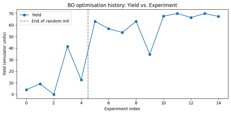
Part 7 — Extension: Multi-Objective Bayesian Optimisation
🧠 Concept: Why multiple objectives?
In the single-objective case we maximised yield alone.
In practice, chemists care about multiple, often conflicting objectives simultaneously:
| Objective | Direction | Chemistry rationale |
|---|---|---|
| Yield | Maximise | More product per reaction |
| TON | Maximise | Higher indicates more stable catalyst |
🧠 Concept: The Pareto Front
When two objectives conflict, there is no single “best” point.
Instead there is a Pareto front — the set of solutions where you cannot improve one objective without worsening another.
Yield
  ▲
  │         ●  ← Pareto optimal (high yield, medium TON)
  │      ●     ← Pareto optimal (medium yield, low TON)
  │   ●        ← Pareto optimal (low yield, very low TON)
  │         ○  ← Dominated (worse than some Pareto point on both objectives)
  └──────────────▶ TON (lower is better)
🧠 Concept: qEHVI — Expected Hypervolume Improvement
qEHVI (Expected Hypervolume Improvement) is the standard acquisition function for multi-objective BO.
It measures how much the current Pareto front’s dominated hypervolume is expected to improve if we run a proposed experiment.
A larger hypervolume = a better Pareto front (it dominates more of the objective space).
⚠️ Computational cost: Multi-objective BO is substantially slower than single-objective BO
because the hypervolume computation scales poorly with the number of Pareto points.
Expect each iteration to take 1–3 minutes on a CPU.
Setting up the multi-objective domain and strategy
We need to:
Add a
TONoutput with aMaximizeObjective.Rebuild the
Domainwith both outputs.Replace
SoboStrategy+qEIwithMoboStrategy+qEHVI.
Everything else (domain inputs, RandomStrategy for initialisation, the ask/tell loop) remains the same.
from bofire.data_models.objectives.api import MinimizeObjective
from bofire.data_models.strategies.api import MoboStrategy
from bofire.data_models.acquisition_functions.api import qEHVI

# ── Objectives ────────────────────────────────────────────────────────────
# MaximizeObjective for yield: higher is better.
max_objective = MaximizeObjective(w=1.0)

# For demonstration purposes only:
# MinimizeObjective: lower is better.
# bounds=[0, 200] tells BOFire the expected range of TON values.
# These bounds are used to normalise TON internally.
min_objective = MinimizeObjective(w=1.0, bounds=[0, 200])

# ── Output features ───────────────────────────────────────────────────────
yield_feature = ContinuousOutput(key="Yield", objective=max_objective)
ton_feature   = ContinuousOutput(key="TON",   objective=max_objective)

# Outputs container now holds BOTH responses.
output_features = Outputs(features=[yield_feature, ton_feature])

# ── Rebuild Domain with multi-objective outputs ───────────────────────────
domain = Domain(
    inputs=input_features,   # Same inputs as before
    outputs=output_features,  # Now includes Yield AND TON
)

# ── Build the MOBO strategy ───────────────────────────────────────────────
# qEHVI : Expected Hypervolume Improvement acquisition function
qExpectedImprovement = qEHVI()

mobo_strategy_data_model = MoboStrategy(
    domain=domain,
    acquisition_function=qExpectedImprovement,
)

# Map to a runnable strategy object.
mobo_strategy = strategies.map(mobo_strategy_data_model)
# ── Random initialisation for MOBO ──────────────────────────────────────
# Same pattern as the single-objective case:
# 1. Build a RandomStrategy on the NEW multi-output domain.
# 2. Ask for 5 random experiments.
# 3. Evaluate them with the emulator (which also returns TON).
# 4. Tell the MOBO strategy so it can fit its initial GP models.
from bofire.data_models.strategies.api import (
RandomStrategy as RandomStrategyModel,
)
random_strategy_model = RandomStrategyModel(domain=domain)
random_strategy = strategies.map(random_strategy_model)
# Ask for 5 random candidates.
candidates = random_strategy.ask(5)
# Evaluate (emulator returns both Yield and TON).
renamed_candidates = candidates.rename(columns=name_map)
renamed_candidates = renamed_candidates.to_dict(orient="records")
print(renamed_candidates)
experiments = []
for candidate in renamed_candidates:
print(candidate)
experiments.append(perform_experiment([candidate]))
print('-------')
flattened = [item for sublist in experiments for item in sublist]
df = pd.DataFrame(flattened)
reverse_name_map = {v: k for k, v in name_map.items()}
experiments = df.rename(columns=reverse_name_map)
# Initialise MOBO strategy with the random data.
# replace=True : start fresh (discard any earlier single-point data)
# retrain=True : fit GPs for both outputs immediately
mobo_strategy.tell(experiments, replace=True, retrain=True)[{'catalyst_loading': 0.5078595930661844, 't_res': 140.4860244998974, 'temperature': 101.81781676512156, 'catalyst': 'P1-L1'}, {'catalyst_loading': 0.6943532584628325, 't_res': 114.6376638500694, 'temperature': 65.88312014768955, 'catalyst': 'P2-L1'}, {'catalyst_loading': 0.7514139146640009, 't_res': 358.9300052429548, 'temperature': 92.64371522816617, 'catalyst': 'P1-L3'}, {'catalyst_loading': 0.7886592444496867, 't_res': 454.8559133789781, 'temperature': 91.56573810882986, 'catalyst': 'P1-L4'}, {'catalyst_loading': 1.9573707962734286, 't_res': 79.78538881098355, 'temperature': 78.51072208231335, 'catalyst': 'P1-L4'}]
{'catalyst_loading': 0.5078595930661844, 't_res': 140.4860244998974, 'temperature': 101.81781676512156, 'catalyst': 'P1-L1'}
[{'catalyst': 'P1-L1', 'catalyst_loading': 0.5078595931, 'iteration': 0, 't_res': 140.4860244999, 'temperature': 101.8178167651, 'ton': 0.0, 'yield': 23.3563842773}]
-------
{'catalyst_loading': 0.6943532584628325, 't_res': 114.6376638500694, 'temperature': 65.88312014768955, 'catalyst': 'P2-L1'}
[{'catalyst': 'P2-L1', 'catalyst_loading': 0.6943532585, 'iteration': 0, 't_res': 114.6376638501, 'temperature': 65.8831201477, 'ton': 0.0, 'yield': 0.0}]
-------
{'catalyst_loading': 0.7514139146640009, 't_res': 358.9300052429548, 'temperature': 92.64371522816617, 'catalyst': 'P1-L3'}
[{'catalyst': 'P1-L3', 'catalyst_loading': 0.7514139147, 'iteration': 0, 't_res': 358.930005243, 'temperature': 92.6437152282, 'ton': 0.0, 'yield': 18.4354839325}]
-------
{'catalyst_loading': 0.7886592444496867, 't_res': 454.8559133789781, 'temperature': 91.56573810882986, 'catalyst': 'P1-L4'}
[{'catalyst': 'P1-L4', 'catalyst_loading': 0.7886592444, 'iteration': 0, 't_res': 454.855913379, 'temperature': 91.5657381088, 'ton': 0.0, 'yield': 42.5867843628}]
-------
{'catalyst_loading': 1.9573707962734286, 't_res': 79.78538881098355, 'temperature': 78.51072208231335, 'catalyst': 'P1-L4'}
[{'catalyst': 'P1-L4', 'catalyst_loading': 1.9573707963, 'iteration': 0, 't_res': 79.785388811, 'temperature': 78.5107220823, 'ton': 0.0, 'yield': 40.7530441284}]
-------
# ── Multi-objective BO loop ───────────────────────────────────────────────
# Identical structure to the single-objective loop.
# The key differences are:
#   - mobo_strategy instead of sobo_strategy
#   - Each ask() step optimises qEHVI (hypervolume improvement) rather than qEI
#   - Each iteration is substantially slower due to the hypervolume calculation
#
# ⚠️  Expect ~1–3 minutes per iteration on a laptop CPU.
# Start with experimental_budget = 5 to confirm it works, then increase.

experimental_budget = 100  # ← Start small; each iteration takes ~1–3 minutes
i = 0
done = False

while not done:
    i += 1
    t1 = time.time()

    # Step 1: Ask for next experiment (maximises expected hypervolume improvement)
    new_candidate = mobo_strategy.ask(1)

    # Step 2: Evaluate with the emulator
    renamed_candidates = new_candidate.rename(columns=name_map)
    renamed_candidates = renamed_candidates.to_dict(orient="records")

    new_experiment = perform_experiment(renamed_candidates)

    df = pd.DataFrame(new_experiment)
    reverse_name_map = {v: k for k, v in name_map.items()}
    new_experiment_df = df.rename(columns=reverse_name_map)

    # Step 3: Update the MOBO strategy with both Yield and TON observations
    mobo_strategy.tell(new_experiment_df)

    print(f"Iteration {i:>3d} | Yield = {new_experiment_df['Yield'].values[0]:.3f} "
          f"| TON = {new_experiment_df['TON'].values[0]:.3f} "
          f"| took {(time.time()-t1):.1f}s")

    if i >= experimental_budget:
        done = True

print("\nMulti-objective optimisation complete!")
/usr/local/lib/python3.12/dist-packages/botorch/acquisition/multi_objective/monte_carlo.py:110: NumericsWarning: qExpectedHypervolumeImprovement has known numerical issues that lead to suboptimal optimization performance. It is strongly recommended to simply replace
qExpectedHypervolumeImprovement --> qLogExpectedHypervolumeImprovement
instead, which fixes the issues and has the same API. See https://arxiv.org/abs/2310.20708 for details.
legacy_ei_numerics_warning(legacy_name=type(self).__name__)
Iteration 1 | Yield = 67.756 | TON = 35.852 | took 23.3s
/usr/local/lib/python3.12/dist-packages/botorch/acquisition/multi_objective/monte_carlo.py:110: NumericsWarning: qExpectedHypervolumeImprovement has known numerical issues that lead to suboptimal optimization performance. It is strongly recommended to simply replace

	 qExpectedHypervolumeImprovement 	 --> 	 qLogExpectedHypervolumeImprovement

instead, which fixes the issues and has the same API. See https://arxiv.org/abs/2310.20708 for details.
  legacy_ei_numerics_warning(legacy_name=type(self).__name__)
Iteration 2 | Yield = 51.982 | TON = 27.129 | took 22.2s
/usr/local/lib/python3.12/dist-packages/botorch/acquisition/multi_objective/monte_carlo.py:110: NumericsWarning: qExpectedHypervolumeImprovement has known numerical issues that lead to suboptimal optimization performance. It is strongly recommended to simply replace

	 qExpectedHypervolumeImprovement 	 --> 	 qLogExpectedHypervolumeImprovement

instead, which fixes the issues and has the same API. See https://arxiv.org/abs/2310.20708 for details.
  legacy_ei_numerics_warning(legacy_name=type(self).__name__)
Iteration 3 | Yield = 82.225 | TON = 44.665 | took 23.8s
/usr/local/lib/python3.12/dist-packages/botorch/acquisition/multi_objective/monte_carlo.py:110: NumericsWarning: qExpectedHypervolumeImprovement has known numerical issues that lead to suboptimal optimization performance. It is strongly recommended to simply replace

	 qExpectedHypervolumeImprovement 	 --> 	 qLogExpectedHypervolumeImprovement

instead, which fixes the issues and has the same API. See https://arxiv.org/abs/2310.20708 for details.
  legacy_ei_numerics_warning(legacy_name=type(self).__name__)
Iteration 4 | Yield = 63.604 | TON = 34.164 | took 25.8s
/usr/local/lib/python3.12/dist-packages/botorch/acquisition/multi_objective/monte_carlo.py:110: NumericsWarning: qExpectedHypervolumeImprovement has known numerical issues that lead to suboptimal optimization performance. It is strongly recommended to simply replace

	 qExpectedHypervolumeImprovement 	 --> 	 qLogExpectedHypervolumeImprovement

instead, which fixes the issues and has the same API. See https://arxiv.org/abs/2310.20708 for details.
  legacy_ei_numerics_warning(legacy_name=type(self).__name__)
Iteration 5 | Yield = 52.623 | TON = 25.722 | took 24.5s
/usr/local/lib/python3.12/dist-packages/botorch/acquisition/multi_objective/monte_carlo.py:110: NumericsWarning: qExpectedHypervolumeImprovement has known numerical issues that lead to suboptimal optimization performance. It is strongly recommended to simply replace

	 qExpectedHypervolumeImprovement 	 --> 	 qLogExpectedHypervolumeImprovement

instead, which fixes the issues and has the same API. See https://arxiv.org/abs/2310.20708 for details.
  legacy_ei_numerics_warning(legacy_name=type(self).__name__)
Iteration 6 | Yield = 85.158 | TON = 43.745 | took 25.5s
/usr/local/lib/python3.12/dist-packages/botorch/acquisition/multi_objective/monte_carlo.py:110: NumericsWarning: qExpectedHypervolumeImprovement has known numerical issues that lead to suboptimal optimization performance. It is strongly recommended to simply replace

	 qExpectedHypervolumeImprovement 	 --> 	 qLogExpectedHypervolumeImprovement

instead, which fixes the issues and has the same API. See https://arxiv.org/abs/2310.20708 for details.
  legacy_ei_numerics_warning(legacy_name=type(self).__name__)
Iteration 7 | Yield = 33.302 | TON = 13.673 | took 27.4s
/usr/local/lib/python3.12/dist-packages/botorch/acquisition/multi_objective/monte_carlo.py:110: NumericsWarning: qExpectedHypervolumeImprovement has known numerical issues that lead to suboptimal optimization performance. It is strongly recommended to simply replace

	 qExpectedHypervolumeImprovement 	 --> 	 qLogExpectedHypervolumeImprovement

instead, which fixes the issues and has the same API. See https://arxiv.org/abs/2310.20708 for details.
  legacy_ei_numerics_warning(legacy_name=type(self).__name__)
Iteration 8 | Yield = 28.264 | TON = 12.093 | took 26.0s
/usr/local/lib/python3.12/dist-packages/botorch/acquisition/multi_objective/monte_carlo.py:110: NumericsWarning: qExpectedHypervolumeImprovement has known numerical issues that lead to suboptimal optimization performance. It is strongly recommended to simply replace

	 qExpectedHypervolumeImprovement 	 --> 	 qLogExpectedHypervolumeImprovement

instead, which fixes the issues and has the same API. See https://arxiv.org/abs/2310.20708 for details.
  legacy_ei_numerics_warning(legacy_name=type(self).__name__)
Iteration 9 | Yield = 74.403 | TON = 36.088 | took 28.5s
/usr/local/lib/python3.12/dist-packages/botorch/acquisition/multi_objective/monte_carlo.py:110: NumericsWarning: qExpectedHypervolumeImprovement has known numerical issues that lead to suboptimal optimization performance. It is strongly recommended to simply replace

	 qExpectedHypervolumeImprovement 	 --> 	 qLogExpectedHypervolumeImprovement

instead, which fixes the issues and has the same API. See https://arxiv.org/abs/2310.20708 for details.
  legacy_ei_numerics_warning(legacy_name=type(self).__name__)
Iteration 10 | Yield = 60.394 | TON = 32.598 | took 28.4s
/usr/local/lib/python3.12/dist-packages/botorch/acquisition/multi_objective/monte_carlo.py:110: NumericsWarning: qExpectedHypervolumeImprovement has known numerical issues that lead to suboptimal optimization performance. It is strongly recommended to simply replace

	 qExpectedHypervolumeImprovement 	 --> 	 qLogExpectedHypervolumeImprovement

instead, which fixes the issues and has the same API. See https://arxiv.org/abs/2310.20708 for details.
  legacy_ei_numerics_warning(legacy_name=type(self).__name__)
Iteration 11 | Yield = 57.824 | TON = 70.427 | took 30.0s
/usr/local/lib/python3.12/dist-packages/botorch/acquisition/multi_objective/monte_carlo.py:110: NumericsWarning: qExpectedHypervolumeImprovement has known numerical issues that lead to suboptimal optimization performance. It is strongly recommended to simply replace

	 qExpectedHypervolumeImprovement 	 --> 	 qLogExpectedHypervolumeImprovement

instead, which fixes the issues and has the same API. See https://arxiv.org/abs/2310.20708 for details.
  legacy_ei_numerics_warning(legacy_name=type(self).__name__)
Part 8 — Analysing the Multi-Objective Results
Visualising the Pareto front
After the MOBO loop, mobo_strategy.experiments contains both Yield and TON for every run.
The most informative visualisation is a 2D scatter plot of TON vs. Yield:
Points on the upper-right frontier (high yield, high TON) approximate the Pareto front.
Points in the lower-left are dominated — there exist experiments that are better on both objectives.
Analysis questions
Can you identify the Pareto-optimal points by eye in the scatter plot?
Is there a visible trade-off (does increasing yield require higher TON)?
How do the multi-objective results compare to the single-objective optimum?
Which catalyst appears most often on the Pareto front?
💡 Extension: Use
bofire’s built-in Pareto front utilities or implement your own filter:
a point (y₁, t₁) dominates (y₂, t₂) ify₁ >= y₂ANDt₁ <= t₂(with at least one strict inequality).
# ── Plot 1: Yield over iterations ────────────────────────────────────────
fig, ax = plt.subplots(figsize=(8, 4))
mobo_strategy.experiments["Yield"].plot(ax=ax, marker="o", linestyle="-", color="steelblue")
ax.axvline(x=4.5, color="gray", linestyle="--", label="End of random init")
ax.set_xlabel("Experiment index")
ax.set_ylabel("Yield")
ax.set_title("MOBO: Yield vs. Experiment Index")
ax.legend()
plt.tight_layout()
plt.show()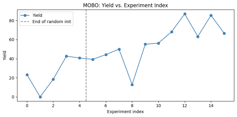
# ── Plot 2: TON over iterations ──────────────────────────────────────────
fig, ax = plt.subplots(figsize=(8, 4))
mobo_strategy.experiments["TON"].plot(ax=ax, marker="s", linestyle="-", color="coral")
ax.axvline(x=4.5, color="gray", linestyle="--", label="End of random init")
ax.set_xlabel("Experiment index")
ax.set_ylabel("TON")
ax.set_title("MOBO: TON vs. Experiment Index")
ax.legend()
plt.tight_layout()
plt.show()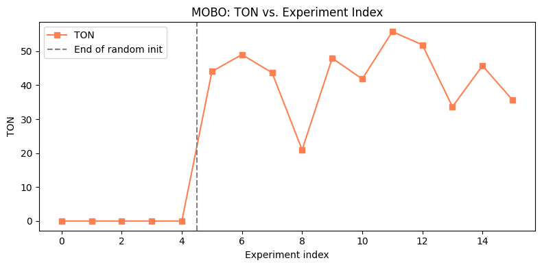
# ── Plot 3: Pareto scatter plot ──────────────────────────────────────────
# This is the most informative MOBO visualisation.
# Each point is one experiment. Points on the upper-left frontier are Pareto-optimal.

df = mobo_strategy.experiments
fig, ax = plt.subplots(figsize=(7, 5))

# Colour-code by iteration index to show how the front evolves.
scatter = ax.scatter(df["Yield"], df["TON"],
                     c=df.index, cmap="viridis", s=60, edgecolors="k", linewidths=0.4)
plt.colorbar(scatter, ax=ax, label="Experiment index")

ax.set_ylabel("TON (lower → less catalyst used)")
ax.set_xlabel("Yield (higher → more product)")
ax.set_title("Multi-Objective BO: Yield vs. TON\n(colour = experiment order)")
plt.tight_layout()
plt.show()

print("\nSummary statistics:")
print(df[["Yield", "TON"]].describe().round(3))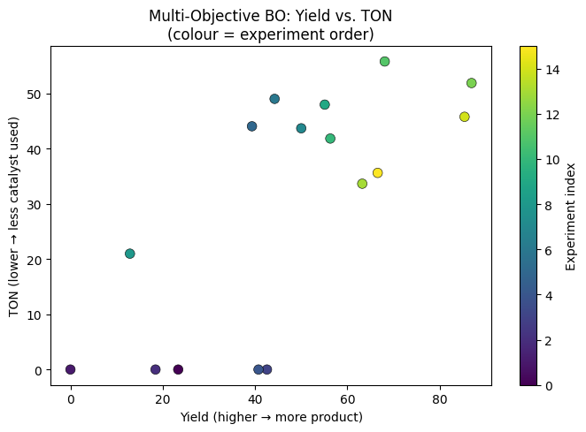
Summary statistics:
        Yield     TON
count  16.000  16.000
mean   47.082  29.384
std    24.759  21.938
min     0.000   0.000
25%    35.342   0.000
50%    47.129  38.714
75%    64.075  46.308
max    86.926  55.777
📝 Summary
In this notebook you have:
Defined a
Domainwith continuous and categorical inputs, and a yield output with aMaximizeObjective.Used a pre-trained neural network emulator as a virtual lab stand-in.
Initialised a GP-based BO strategy with random experiments.
Implemented the ask–evaluate–tell loop for single-objective BO.
Interpreted the optimisation history and identified the best conditions.
Extended the setup to multi-objective BO with
MoboStrategyandqEHVI.Visualised the Pareto front showing the yield–TON trade-off.
Further reading
Shields, B.J. et al. Bayesian reaction optimisation as a tool for chemical synthesis. Nature 590, 89–96 (2021).
Hernández-Lobato, J.M. et al. Predictive Entropy Search for Multi-objective Bayesian Optimization. NeurIPS 2016.