Visualizing BO for a synthetic example
This notebook is a modified version of the notebook associated with ❝Bayesian optimization of nanoporous materials❞ A. Deshwal, C. Simon, J. R. Doppa. Molecular Systems Design & Engineering. (2021).
First, we will install all of the necessary packages:
! pip install torch numpy matplotlib gpytorch botorch seabornRequirement already satisfied: torch in /home/bogosort/work/teaching/2024-BO-summer-school/main/.venv/lib/python3.10/site-packages (2.4.1)
Requirement already satisfied: numpy in /home/bogosort/work/teaching/2024-BO-summer-school/main/.venv/lib/python3.10/site-packages (1.26.4)
Requirement already satisfied: matplotlib in /home/bogosort/work/teaching/2024-BO-summer-school/main/.venv/lib/python3.10/site-packages (3.9.2)
Requirement already satisfied: gpytorch in /home/bogosort/work/teaching/2024-BO-summer-school/main/.venv/lib/python3.10/site-packages (1.12)
Requirement already satisfied: botorch in /home/bogosort/work/teaching/2024-BO-summer-school/main/.venv/lib/python3.10/site-packages (0.11.3)
Requirement already satisfied: filelock in /home/bogosort/work/teaching/2024-BO-summer-school/main/.venv/lib/python3.10/site-packages (from torch) (3.15.4)
Requirement already satisfied: typing-extensions>=4.8.0 in /home/bogosort/work/teaching/2024-BO-summer-school/main/.venv/lib/python3.10/site-packages (from torch) (4.12.2)
Requirement already satisfied: sympy in /home/bogosort/work/teaching/2024-BO-summer-school/main/.venv/lib/python3.10/site-packages (from torch) (1.13.2)
Requirement already satisfied: networkx in /home/bogosort/work/teaching/2024-BO-summer-school/main/.venv/lib/python3.10/site-packages (from torch) (2.8.8)
Requirement already satisfied: jinja2 in /home/bogosort/work/teaching/2024-BO-summer-school/main/.venv/lib/python3.10/site-packages (from torch) (3.1.4)
Requirement already satisfied: fsspec in /home/bogosort/work/teaching/2024-BO-summer-school/main/.venv/lib/python3.10/site-packages (from torch) (2024.9.0)
Requirement already satisfied: nvidia-cuda-nvrtc-cu12==12.1.105 in /home/bogosort/work/teaching/2024-BO-summer-school/main/.venv/lib/python3.10/site-packages (from torch) (12.1.105)
Requirement already satisfied: nvidia-cuda-runtime-cu12==12.1.105 in /home/bogosort/work/teaching/2024-BO-summer-school/main/.venv/lib/python3.10/site-packages (from torch) (12.1.105)
Requirement already satisfied: nvidia-cuda-cupti-cu12==12.1.105 in /home/bogosort/work/teaching/2024-BO-summer-school/main/.venv/lib/python3.10/site-packages (from torch) (12.1.105)
Requirement already satisfied: nvidia-cudnn-cu12==9.1.0.70 in /home/bogosort/work/teaching/2024-BO-summer-school/main/.venv/lib/python3.10/site-packages (from torch) (9.1.0.70)
Requirement already satisfied: nvidia-cublas-cu12==12.1.3.1 in /home/bogosort/work/teaching/2024-BO-summer-school/main/.venv/lib/python3.10/site-packages (from torch) (12.1.3.1)
Requirement already satisfied: nvidia-cufft-cu12==11.0.2.54 in /home/bogosort/work/teaching/2024-BO-summer-school/main/.venv/lib/python3.10/site-packages (from torch) (11.0.2.54)
Requirement already satisfied: nvidia-curand-cu12==10.3.2.106 in /home/bogosort/work/teaching/2024-BO-summer-school/main/.venv/lib/python3.10/site-packages (from torch) (10.3.2.106)
Requirement already satisfied: nvidia-cusolver-cu12==11.4.5.107 in /home/bogosort/work/teaching/2024-BO-summer-school/main/.venv/lib/python3.10/site-packages (from torch) (11.4.5.107)
Requirement already satisfied: nvidia-cusparse-cu12==12.1.0.106 in /home/bogosort/work/teaching/2024-BO-summer-school/main/.venv/lib/python3.10/site-packages (from torch) (12.1.0.106)
Requirement already satisfied: nvidia-nccl-cu12==2.20.5 in /home/bogosort/work/teaching/2024-BO-summer-school/main/.venv/lib/python3.10/site-packages (from torch) (2.20.5)
Requirement already satisfied: nvidia-nvtx-cu12==12.1.105 in /home/bogosort/work/teaching/2024-BO-summer-school/main/.venv/lib/python3.10/site-packages (from torch) (12.1.105)
Requirement already satisfied: triton==3.0.0 in /home/bogosort/work/teaching/2024-BO-summer-school/main/.venv/lib/python3.10/site-packages (from torch) (3.0.0)
Requirement already satisfied: nvidia-nvjitlink-cu12 in /home/bogosort/work/teaching/2024-BO-summer-school/main/.venv/lib/python3.10/site-packages (from nvidia-cusolver-cu12==11.4.5.107->torch) (12.6.68)
Requirement already satisfied: contourpy>=1.0.1 in /home/bogosort/work/teaching/2024-BO-summer-school/main/.venv/lib/python3.10/site-packages (from matplotlib) (1.3.0)
Requirement already satisfied: cycler>=0.10 in /home/bogosort/work/teaching/2024-BO-summer-school/main/.venv/lib/python3.10/site-packages (from matplotlib) (0.12.1)
Requirement already satisfied: fonttools>=4.22.0 in /home/bogosort/work/teaching/2024-BO-summer-school/main/.venv/lib/python3.10/site-packages (from matplotlib) (4.53.1)
Requirement already satisfied: kiwisolver>=1.3.1 in /home/bogosort/work/teaching/2024-BO-summer-school/main/.venv/lib/python3.10/site-packages (from matplotlib) (1.4.7)
Requirement already satisfied: packaging>=20.0 in /home/bogosort/work/teaching/2024-BO-summer-school/main/.venv/lib/python3.10/site-packages (from matplotlib) (24.1)
Requirement already satisfied: pillow>=8 in /home/bogosort/work/teaching/2024-BO-summer-school/main/.venv/lib/python3.10/site-packages (from matplotlib) (10.4.0)
Requirement already satisfied: pyparsing>=2.3.1 in /home/bogosort/work/teaching/2024-BO-summer-school/main/.venv/lib/python3.10/site-packages (from matplotlib) (3.1.4)
Requirement already satisfied: python-dateutil>=2.7 in /home/bogosort/work/teaching/2024-BO-summer-school/main/.venv/lib/python3.10/site-packages (from matplotlib) (2.9.0.post0)
Requirement already satisfied: mpmath<=1.3,>=0.19 in /home/bogosort/work/teaching/2024-BO-summer-school/main/.venv/lib/python3.10/site-packages (from gpytorch) (1.3.0)
Requirement already satisfied: scikit-learn in /home/bogosort/work/teaching/2024-BO-summer-school/main/.venv/lib/python3.10/site-packages (from gpytorch) (1.5.1)
Requirement already satisfied: scipy in /home/bogosort/work/teaching/2024-BO-summer-school/main/.venv/lib/python3.10/site-packages (from gpytorch) (1.14.1)
Requirement already satisfied: linear-operator>=0.5.2 in /home/bogosort/work/teaching/2024-BO-summer-school/main/.venv/lib/python3.10/site-packages (from gpytorch) (0.5.2)
Requirement already satisfied: multipledispatch in /home/bogosort/work/teaching/2024-BO-summer-school/main/.venv/lib/python3.10/site-packages (from botorch) (1.0.0)
Requirement already satisfied: pyro-ppl>=1.8.4 in /home/bogosort/work/teaching/2024-BO-summer-school/main/.venv/lib/python3.10/site-packages (from botorch) (1.9.1)
Requirement already satisfied: jaxtyping>=0.2.9 in /home/bogosort/work/teaching/2024-BO-summer-school/main/.venv/lib/python3.10/site-packages (from linear-operator>=0.5.2->gpytorch) (0.2.34)
Requirement already satisfied: typeguard~=2.13.3 in /home/bogosort/work/teaching/2024-BO-summer-school/main/.venv/lib/python3.10/site-packages (from linear-operator>=0.5.2->gpytorch) (2.13.3)
Requirement already satisfied: opt-einsum>=2.3.2 in /home/bogosort/work/teaching/2024-BO-summer-school/main/.venv/lib/python3.10/site-packages (from pyro-ppl>=1.8.4->botorch) (3.3.0)
Requirement already satisfied: pyro-api>=0.1.1 in /home/bogosort/work/teaching/2024-BO-summer-school/main/.venv/lib/python3.10/site-packages (from pyro-ppl>=1.8.4->botorch) (0.1.2)
Requirement already satisfied: tqdm>=4.36 in /home/bogosort/work/teaching/2024-BO-summer-school/main/.venv/lib/python3.10/site-packages (from pyro-ppl>=1.8.4->botorch) (4.66.5)
Requirement already satisfied: six>=1.5 in /home/bogosort/work/teaching/2024-BO-summer-school/main/.venv/lib/python3.10/site-packages (from python-dateutil>=2.7->matplotlib) (1.16.0)
Requirement already satisfied: MarkupSafe>=2.0 in /home/bogosort/work/teaching/2024-BO-summer-school/main/.venv/lib/python3.10/site-packages (from jinja2->torch) (2.1.5)
Requirement already satisfied: joblib>=1.2.0 in /home/bogosort/work/teaching/2024-BO-summer-school/main/.venv/lib/python3.10/site-packages (from scikit-learn->gpytorch) (1.4.2)
Requirement already satisfied: threadpoolctl>=3.1.0 in /home/bogosort/work/teaching/2024-BO-summer-school/main/.venv/lib/python3.10/site-packages (from scikit-learn->gpytorch) (3.5.0)
import math
import torch
import gpytorch
from matplotlib import pyplot as plt
import seaborn as sns
import botorch

%matplotlib inline
%load_ext autoreload
%autoreload 2
import numpy as np
from botorch.acquisition.analytic import ExpectedImprovement
from torch.distributions import Normal
Let’s make our plots pretty :)
cool_colors = ['#00BEFF', '#D4CA3A', '#FF6DAE', '#67E1B5', '#EBACFA', '#9E9E9E', '#F1988E', '#5DB15A', '#E28544', '#52B8AA']
# cool_colors = sns.color_palette("Set2")
We’ll define the underlying objective function.
Recall, this example is purely for demonstrative purposes -- in practice, we would not know this functional form.
def f(x):
    return x * torch.exp(-4*x) + torch.sin(3*x*math.pi)*torch.exp(-2* x)# + torch.atan(0.7*math.pi*x)#* torch.exp(-2*x) + 0.3 * torch.sin(3*math.pi*x)
#torch.sin(x * (3.2 * math.pi)) * torch.exp(-1.0*x) * np.cos(x*math.pi) + 0.9*torch.exp(-8*(x - 0.4) ** 2)# + np.exp(-x)
#     return torch.exp(-6*(x - 0.2) ** 2)# + np.exp(-x)


plt.figure()
x = torch.linspace(0, 1, 100)
plt.plot(x, f(x))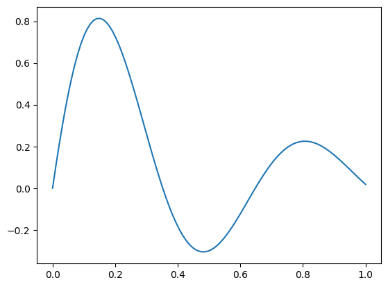
First, we’ll generate some points for
## Underlying true ('ground') objective
ground_x = torch.linspace(0, 1, 100)
# True function is sin(2*pi*x) with Gaussian noise
# ground_y = f(ground_x)
ground_y = f(ground_x)# torch.sin(ground_x * (2 * math.pi)) * torch.exp(-0.1 * ground_x) - (ground_x - 0.2) ** 2
# Generating initial training data
torch.manual_seed(1) # seed for reproducibility
# Training data 5 points selected
train_x = torch.tensor([0.01, 0.25, 0.45, 0.6, 0.93])
# True function is sin(2*pi*x) with Gaussian noise
train_y = f(train_x)# np.sin(train_x * (2 * math.pi)) * np.exp(-0.1 * train_x) - (train_x - 0.) ** 2 #+ torch.randn(train_x.size()) * math.sqrt(0.02)
# train_y = np.sin(train_x * (2 * math.pi)) * np.exp(-0.1 * train_x) - 4* (train_x - 0.2) ** 2# simple GP model, exact inference
class ExactGPModel(gpytorch.models.ExactGP):
def __init__(self, train_x, train_y, likelihood):
super(ExactGPModel, self).__init__(train_x, train_y, likelihood)
self.mean_module = gpytorch.means.ConstantMean()
self.covar_module = gpytorch.kernels.ScaleKernel(gpytorch.kernels.RBFKernel())
def forward(self, x):
mean_x = self.mean_module(x)
covar_x = self.covar_module(x)
return gpytorch.distributions.MultivariateNormal(mean_x, covar_x)
# initialize likelihood and model
likelihood = gpytorch.likelihoods.GaussianLikelihood()
likelihood.noise_covar.noise = 1e-4 # sets the value to zero
likelihood.noise_covar.raw_noise.requires_grad = False # optimizer won't optimize noise hyper-parameter.
model = ExactGPModel(train_x, train_y, likelihood)# Fitting of the model with training set
model.train()
likelihood.train()
# Use the adam optimizer
optimizer = torch.optim.Adam([
{'params': model.parameters()},
], lr=0.1)
# "Loss" for GPs - the marginal log likelihood
mll = gpytorch.mlls.ExactMarginalLogLikelihood(likelihood, model)
training_iter = 100
for i in range(training_iter):
# Zero gradients from previous iteration
optimizer.zero_grad()
# Output from model
output = model(train_x)
# Calc loss and backprop gradients
loss = -mll(output, train_y)
loss.backward()
optimizer.step()
# fit_gpytorch_model(mll)# Plotting Figure 3 in the paper
model.eval()
likelihood.eval()
# Test points are regularly spaced along [0,1]
# Make predictions by feeding model through likelihood
with torch.no_grad(), gpytorch.settings.fast_pred_var():
test_x = torch.linspace(0, 1, 100)
observed_pred = likelihood(model(test_x))
with torch.no_grad():
# Initialize plot
# Get upper and lower confidence bounds
lower, upper = observed_pred.confidence_region()
# Plot training data as black stars
plt.scatter(train_x.numpy(), train_y.numpy(), marker="+", color="k", label='observations $\{(x_i, y_i)\}$', s=95, zorder=2000, lw=5)
plt.plot(ground_x.numpy(), ground_y.numpy(), linestyle="--", color=cool_colors[2], label='truth, $f(x)$', lw=3)
# Plot predictive means as blue line
plt.plot(test_x.numpy(), observed_pred.mean.numpy(), color=cool_colors[0], label='model, $\hat{y}(x)$', lw=3)
# Shade between the lower and upper confidence bounds
plt.fill_between(test_x.numpy(), lower.numpy(), upper.numpy(), alpha=0.15, color=cool_colors[0], edgecolor="none")
# plt.ylim(the_ylims)
plt.xlim([0, 1])
plt.xlabel('NPM feature space, $x$', fontsize=15)
plt.ylabel('property, $y$', fontsize=15)
plt.yticks([])
plt.xticks([])
plt.legend(fontsize=12)
the_ylims = plt.gca().get_ylim()
plt.savefig("gp_example.pdf")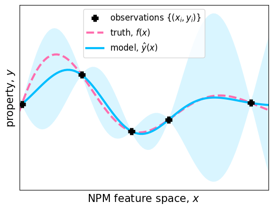
with torch.no_grad():
    # Initialize plot
    # Get upper and lower confidence bounds
    lower, upper = observed_pred.confidence_region()
    fig = plt.figure()
    # Plot training data as black stars
    plt.scatter(train_x.numpy(), train_y.numpy(), marker="+", color="k", label='observations $\{(x_i, y_i)\}$', s=95, zorder=2000, lw=5)
#     plt.plot(ground_x.numpy(), ground_y.numpy(), linestyle="--", color=cool_colors[2], label='truth, $f(x)$', lw=3)
    # Plot predictive means as blue line
    plt.plot(test_x.numpy(), observed_pred.mean.numpy(), color=cool_colors[0], label='model, $\hat{y}(x)$', lw=3)
    # Shade between the lower and upper confidence bounds
    plt.fill_between(test_x.numpy(), lower.numpy(), upper.numpy(), alpha=0.15, color=cool_colors[0], edgecolor="none")
#     plt.ylim(the_ylims)
    plt.xlim([0, 1])
#     plt.xlabel('NPM feature space, $x$', fontsize=15)
#     plt.ylabel('property, $y$', fontsize=15)
    fig.patch.set_visible(False)
    plt.gca().axis('off')
    plt.yticks([])
    plt.xticks([])
#     plt.legend(fontsize=12)
    the_ylims = plt.gca().get_ylim()
    plt.savefig("gp_example_for_illustration.pdf")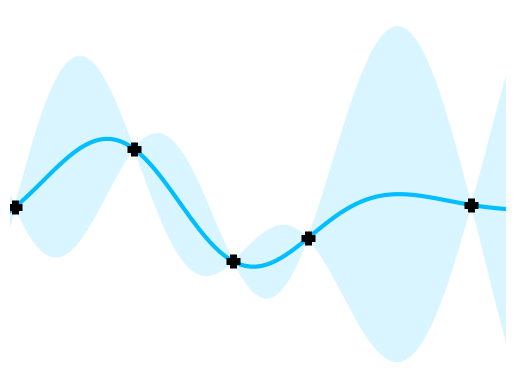
the_ylims(-1.133509135246277, 1.5233301877975465)#### computing expected improvement objective for test points
posterior = model(test_x)
mean = posterior.mean
sigma = posterior.variance.clamp_min(1e-9).sqrt()#.view(view_shape)
u = (mean - torch.max(train_y).expand_as(mean)) / sigma
normal = Normal(torch.zeros_like(u), torch.ones_like(u))
ucdf = normal.cdf(u)
updf = torch.exp(normal.log_prob(u))
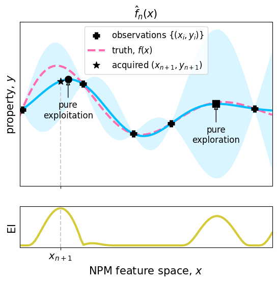
ei = sigma * (updf + u * ucdf)# Plotting figure 4 (a)
with torch.no_grad():
# Get upper and lower confidence bounds
lower, upper = observed_pred.confidence_region()
fig, axs = plt.subplots(2, 1, gridspec_kw={'height_ratios': [4, 1]}, figsize=[6.4, 1.2*4.8], sharex=True)
# Plot training data as black stars
axs[0].scatter(train_x.numpy(), train_y.numpy(), marker="+", color="k", label='observations $\{(x_i, y_i)\}$', s=95, zorder=2000, lw=5)
axs[0].plot(ground_x.numpy(), ground_y.numpy(), linestyle="--", color=cool_colors[2], label='truth, $f(x)$', lw=3)
# Plot predictive means as blue line
axs[0].plot(test_x.numpy(), observed_pred.mean.numpy(), color=cool_colors[0], lw=3)
# Shade between the lower and upper confidence bounds
axs[0].fill_between(test_x.numpy(), lower.numpy(), upper.numpy(), alpha=0.15, color=cool_colors[0], edgecolor="none")
axs[1].plot(test_x.numpy(), 2*(ei.numpy())-3, 'g', label='Expected Improvement (EI)', lw=3, color=cool_colors[1])
xy_exploitation = (test_x[torch.argmax(observed_pred.mean)].numpy(), observed_pred.mean[torch.argmax(observed_pred.mean)].numpy())
axs[0].scatter(xy_exploitation[0], xy_exploitation[1], color="k", s=95, marker="o", zorder=1000)
ann = axs[0].annotate("pure\nexploitation",
xy=xy_exploitation, xycoords='data',
xytext=(xy_exploitation[0], xy_exploitation[1]-0.5),
# xytext=(0.3, 1.0),
textcoords='data',
size=12, va="center", ha="center",
arrowprops=dict(arrowstyle="-|>",
fc=cool_colors[5], ec="k"), zorder=100000
)
xy_exploration = (test_x[torch.argmax(observed_pred.stddev)].numpy(), observed_pred.mean[torch.argmax(observed_pred.stddev)].numpy())
axs[0].scatter(xy_exploration[0], xy_exploration[1], color="k", s=95, marker="s", zorder=1000)
ann = axs[0].annotate("pure\nexploration",
xy=xy_exploration, xycoords='data',
xytext=(xy_exploration[0], xy_exploration[1]-0.5), textcoords='data',
size=12, va="center", ha="center",
arrowprops=dict(arrowstyle="-|>",
fc=cool_colors[5], ec="k"), zorder=100000
)
axs[0].scatter(test_x[torch.argmax(ei)].numpy(), observed_pred.mean[torch.argmax(ei)].numpy(), color="k", label='acquired $(x_{n+1}, y_{n+1})$', s=95, marker="*", zorder=1000)
axs[0].set_ylim(the_ylims)
axs[1].set_xlabel('NPM feature space, $x$', fontsize=15)
axs[0].set_ylabel('property, $y$', fontsize=15)
axs[1].set_ylabel('EI', fontsize=15)
for ax in axs:
ax.set_yticks([])
ax.set_xticks([])
ax.set_xlim([0, 1])
axs[1].axvline(x=test_x[torch.argmax(ei)].numpy(), linestyle="--", color="0.8")
axs[0].plot([test_x[torch.argmax(ei)].numpy() for i in range(2)], [axs[0].get_ylim()[0], observed_pred.mean[torch.argmax(ei)].numpy()], linestyle="--", color="0.8")
axs[0].set_title('$\hat{f}_{n}(x)$', fontsize=15)
axs[0].set_xticks([test_x[torch.argmax(ei)].numpy()])
axs[1].set_xticklabels(["$x_{n+1}$"])
axs[1].tick_params(axis='x', which='major', labelsize=14)
axs[0].legend(fontsize=12)#['Expected Improvement'])
plt.savefig("gp_ei_iteration_n.pdf")/tmp/ipykernel_3421885/2727657776.py:14: UserWarning: color is redundantly defined by the 'color' keyword argument and the fmt string "g" (-> color=(0.0, 0.5, 0.0, 1)). The keyword argument will take precedence.
axs[1].plot(test_x.numpy(), 2*(ei.numpy())-3, 'g', label='Expected Improvement (EI)', lw=3, color=cool_colors[1])
## update training set with new point (one with highest EI value)
new_train_x = torch.cat([train_x, test_x[torch.argmax(ei)].unsqueeze(0)])
new_train_y = f(new_train_x)# torch.sin(new_train_x * (2 * math.pi)) #+ torch.randn(new_train_x.size()) * math.sqrt(0.04)
## Fit the model
likelihood = gpytorch.likelihoods.GaussianLikelihood()
likelihood.noise_covar.noise = 1e-4 # sets the value to zero
likelihood.noise_covar.raw_noise.requires_grad = False # optimizer won't optimize noise hyper-parameter.
model = ExactGPModel(new_train_x, new_train_y, likelihood)
# Find optimal model hyperparameters
model.train()
likelihood.train()
# Use the adam optimizer
optimizer = torch.optim.Adam([
{'params': model.parameters()}, # Includes GaussianLikelihood parameters
], lr=0.1)
# "Loss" for GPs - the marginal log likelihood
mll = gpytorch.mlls.ExactMarginalLogLikelihood(likelihood, model)
training_iter = 100
for i in range(training_iter):
# Zero gradients from previous iteration
optimizer.zero_grad()
# Output from model
output = model(new_train_x)
# Calc loss and backprop gradients
loss = -mll(output, new_train_y)
loss.backward()
# print('Iter %d/%d - Loss: %.3f lengthscale: %.3f noise: %.3f' % (
# i + 1, training_iter, loss.item(),
# model.covar_module.base_kernel.lengthscale.item(),
# model.likelihood.noise.item()
# ))
optimizer.step()#### computing expected improvement objective for test points
mean = posterior.mean
sigma = posterior.variance.clamp_min(1e-9).sqrt()#.view(view_shape)
u = (mean - torch.max(new_train_y).expand_as(mean)) / sigma
normal = Normal(torch.zeros_like(u), torch.ones_like(u))
ucdf = normal.cdf(u)
updf = torch.exp(normal.log_prob(u))
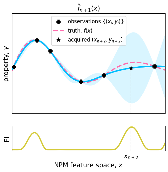
ei = sigma * (updf + u * ucdf)## Plotting figure 4(b)
model.eval()
likelihood.eval()
observed_pred = likelihood(model(test_x))
with torch.no_grad():
# Initialize plot
# Get upper and lower confidence bounds
lower, upper = observed_pred.confidence_region()
fig, axs = plt.subplots(2, 1, gridspec_kw={'height_ratios': [4, 1]}, figsize=[6.4, 1.2*4.8], sharex=True)
# Plot training data as black stars
# Plot training data as black stars
axs[0].scatter(new_train_x.numpy(), new_train_y.numpy(), marker="+", color="k", label='observations $\{(x_i, y_i)\}$', s=95, zorder=2000, lw=5)
axs[0].plot(ground_x.numpy(), ground_y.numpy(), linestyle="--", color=cool_colors[2], label='truth, $f(x)$', lw=3)
# Plot predictive means as blue line
axs[0].plot(test_x.numpy(), observed_pred.mean.numpy(), color=cool_colors[0], lw=3)
# axs[0].scatter(new_train_x.numpy(), new_train_y.numpy(), marker="+", color="k", label='observation $(x_i, y_i)$', s=95, zorder=2000, lw=5)
# axs[0].plot(ground_x.numpy(), ground_y.numpy(),'r--', label='True property')
# Plot predictive means as blue line
axs[0].plot(test_x.numpy(), observed_pred.mean.numpy(), color=cool_colors[0], lw=3)
# Shade between the lower and upper confidence bounds
axs[0].fill_between(test_x.numpy(), lower.numpy(), upper.numpy(), alpha=0.15, color=cool_colors[0], edgecolor="none")
axs[0].set_ylim(the_ylims)
axs[1].set_xlabel('NPM feature space, $x$', fontsize=15)
axs[0].set_ylabel('property, $y$', fontsize=15)
axs[1].set_ylabel('EI', fontsize=15)
for ax in axs:
ax.set_yticks([])
ax.set_xticks([])
ax.set_xlim([0, 1])
axs[0].scatter(test_x[torch.argmax(ei)].numpy(), observed_pred.mean[torch.argmax(ei)].numpy(), color="k", label='acquired $(x_{n+2}, y_{n+2})$', s=95, marker="*", zorder=1000)
axs[1].axvline(x=test_x[torch.argmax(ei)].numpy(), linestyle="--", color="0.8")
axs[0].plot([test_x[torch.argmax(ei)].numpy() for i in range(2)], [axs[0].get_ylim()[0], observed_pred.mean[torch.argmax(ei)].numpy()], linestyle="--", color="0.8")
axs[0].set_title('$\hat{f}_{n+1}(x)$', fontsize=15)
axs[0].set_xticks([test_x[torch.argmax(ei)].numpy()])
axs[1].set_xticklabels(["$x_{n+2}$"])
axs[1].tick_params(axis='x', which='major', labelsize=14)
axs[1].plot(test_x.numpy(), 2*(ei.numpy())-3, 'g', label='Expected Improvement (EI)', lw=3, color=cool_colors[1])
axs[0].legend(fontsize=12)#['Expected Improvement'])
plt.savefig("gp_ei_iteration_np1.pdf")/tmp/ipykernel_3421885/3783663021.py:38: UserWarning: color is redundantly defined by the 'color' keyword argument and the fmt string "g" (-> color=(0.0, 0.5, 0.0, 1)). The keyword argument will take precedence.
axs[1].plot(test_x.numpy(), 2*(ei.numpy())-3, 'g', label='Expected Improvement (EI)', lw=3, color=cool_colors[1])