Tutorial on Basics of Machine Learning in Computational Molecular Science

Tutorial on Basics of Machine Learning in Computational Molecular Science#

Prelude#

This tutorial is a basic introduction into machine learning (ML) workflows in the context of molecular simulation and computational materials research. The notebook introduces workflows and concepts related to

Data preparation and analysis
Generating chemical representations and features
Dimensionality Reduction
Clustering
Kernel-based model fitting
Hyperparameter Optimization
Uncertainty Quantification

The required dependencies include

Atomic Simulation Environment (ase): We will use this to store molecular structures and properties
scikit-learn: machine learning library
dscribe: library to generate molecular representations (descriptors)
openTSNE

As you go through the notebook and work through the tasks, look through the documentation pages of those packages if you get stuck.

We will be working on two datasets of molecules, one that explores composition space (dataset of different molecules), and one that explores configurational space (data from molecular dynamics):

Dataset of five short molecular dynamics trajectories of cyclohexane, Courtesy of “Quantum Chemistry in the Age of Machine Learning”, edited by Pavlo Dral (2022)
The QM7 dataset of organic molecules with up to 7 non-hydrogen atoms, Courtesy of Rupp et al., Phys. Rev. Lett. 108, 058301 (2012) and qmlcode.org

Both datasets feature structures and energies.

Reinhard Maurer, University of Warwick (2025)

# only if you run in google colab

# import locale
# locale.getpreferredencoding = lambda: "UTF-8"

# ! pip install ase scikit-learn dcribe opentsne data-tutorials
# get_ipython().kernel.do_shutdown(restart=True)

# get the data

#basic stuff
import os
import sys
from functools import partial
import numpy as np
import ase
import random
from ase.io import read, write
from ase.visualize import view
from matplotlib import pyplot as plt
import matplotlib as mpl
import pandas
import seaborn as sns
from ase.build import molecule
from weas_widget import WeasWidget

#ML stuff
import dscribe
import sklearn
from sklearn.metrics.pairwise import pairwise_kernels
from sklearn.model_selection import train_test_split
from tqdm.auto import tqdm # progress bars for loops

%matplotlib inline

Part 1: Data Preparation and Analysis#

Let’s start with a dataset of five short MD simulations of different conformers of cyclohexane.

We start five independent simulations initialized within each of the known cyclohexane conformers shown in the below figure. The MD simulations were run for 10,000 time steps each. The data contains the atom positions, velocities, energies and forces. These types of MD simulations will explore the energy landscape and settle within local and/or global minima.

cyclehexane conformers

Read and analyse Molecular Dynamics Data#

# read in the frames from each MD simulation
traj = []
names = ['chair', 'twist-boat', 'boat', 'half-chair', 'planar']
rgb_colors = [(0.13333333333333333, 0.47058823529411764, 0.7098039215686275),
                (0.4588235294117647, 0.7568627450980392, 0.34901960784313724),
                (0.803921568627451, 0.6078431372549019, 0.16862745098039217),
                (0.803921568627451, 0.13725490196078433, 0.15294117647058825),
                (0.4392156862745098, 0.2784313725490196, 0.611764705882353),]

ranges = np.zeros((len(names), 2), dtype=int)
conf_idx = np.zeros(len(names), dtype=int)

for i, n in enumerate(names):
    frames = read(f'./cyclohexane_data/MD/{n}.xyz', '::')

    for frame in frames:
        # wrap each frame in its box
        frame.wrap(eps=1E-10)

        # mask each frame so that descriptors are only centered on carbon (#6) atoms
        mask = np.zeros(len(frame))
        mask[np.where(frame.numbers == 6)[0]] = 1
        frame.arrays['center_atoms_mask'] = mask

    ranges[i] = (len(traj), len(traj) + len(frames)) #list of data ranges
    conf_idx[i] = len(traj) # handy list to indicate the index of the first frame for each trajectory
    traj = [*traj, *frames] # full list of frames, 50000 entries

After this call, all the MD frames of the 5 different runs sit in the object traj. traj is a list of ASE Atoms objects, which contain the structure definition, positions, velocities, energies etc.

If you are unfamiliar with ASE, please explore the online documentation and play around a bit with it in the following cells.

You can see, we have 50,000 configurations, each labeled with an energy in electronvolt (eV).

Task for you

Visualize the trajectories of the 5 different molecules and study their different configurations and dynamics.

#pick a molecule to visualize its trajectory
# ['chair', 'twist-boat', 'boat', 'half-chair', 'planar']
molecule = 'chair'
########
i = names.index(molecule)
r = ranges[i]
mol_traj = traj[r[0]:r[1]]

print("Visualizing '{0}' trajectory".format(molecule))
# visualize the trajectory of the molecule
viewer = WeasWidget()
viewer.from_ase(mol_traj)
viewer.avr.model_style = 1
viewer.avr.show_hydrogen_bonds = True
viewer

Next, we plot the energy as a function of time along the trajectory.

# energies of the simulation frames
energy = np.array([a.info['energy_eV'] for a in traj])

# energies of the known conformers
c_energy = np.array([traj[c].info['energy_eV'] for c in conf_idx])

# extrema for the energies
max_e = max(energy)
min_e = min(energy)

print('energy range goes from {0:10.6f} to {1:10.6f} eV'.format(min_e, max_e))

fig, ax = plt.subplots(1, figsize=(3*4.8528, 3*1.2219))

for n, c, r, rgb in zip(names, c_energy, ranges, rgb_colors):
    ax.plot(range(0, r[1] - r[0]),
            energy[r[0]:r[1]] - min_e,
            label=n,
            c=rgb,
            zorder=-1)
    
ax.legend()
ax.set_xlabel("Simulation Timestep")
ax.set_ylabel("Energy in eV")

ax.set_xlim([0, len(energy)//5])
ax.set_ylim([-0.1, 1.25 * (max_e - min_e)])
ax.set_yticklabels([])

plt.tight_layout()
plt.savefig('energy.png')
plt.show()

We can see that most trajectories appear relatively stable in their configuration, but the ‘planar’ configuration seems to change its configuration relatively quickly to one of the others.

Task for you

The five simulations convergence into two different conformers, the chair conformer and the twist-boat conformer. Can you tell which simulation converges into which configuration? (This is doable the old-fashioned way by visually inspecting the MD simulations or by using machine learning methods.)
Make a note of this as it will help you to rationalise some of the later findings.

Read and analyse QM7 molecule dataset#

The QM7 dataset contains 7101 molecules with up to 7 non-hydrogen atoms. It is one of the first datasets that was studied when the idea of “quantum machine learning” came up, so machine learning regression of quantum chemistry properties based on feature representations that correlate well with molecular structure and properties.

For each of the 7101 molecules, we have 2 labels:

PBE0/def2-TZVP atomization energy in eV (energy_eV)
and the difference between PBE0 and DFTB3 atomization energy in eV (delta_energy_eV)

Reading the database can take up to two minutes, so please be patient.

def get_qm7_energies(filename, key="dft"):
    """ Returns a dictionary with heats of formation for each xyz-file.
    """

    f = open(filename, "r")
    lines = f.readlines()
    f.close()

    energies = []

    for line in lines:
        tokens = line.split()

        xyz_name = tokens[0]
        hof = float(tokens[1])
        dftb = float(tokens[2])

        if key=="delta":
            energies.append(hof - dftb)
        else:
            energies.append(hof)

    return energies

# Import QM7, already parsed to QML
from ase.io import read

qm7_dft_energy = get_qm7_energies("hof_qm7.txt", key="dft")
qm7_delta_energy = get_qm7_energies("hof_qm7.txt", key = "delta")

qm7 = [read("qm7/"+f) for f in sorted(os.listdir("qm7/"))]

Let’s visualize some of those more than 7000 molecules. You will quickly see that the database also contains some rather strange ones …

mol = qm7[21]
print(mol)
viewer = WeasWidget()
viewer.from_ase(mol)
viewer.avr.model_style = 1
viewer.avr.show_hydrogen_bonds = True
viewer

#lets attach the labels to the ASE objects as we did in the previous dataset
for i, mol in enumerate(qm7):
    mol.info["energy_eV"] = qm7_dft_energy[i]         # PBE0/def2-TZVP atomization energy in eV
    mol.info["energy_delta_eV"] = qm7_delta_energy[i] # difference between PBE0 and DFTB3 atomization energy in eV

random.seed(42)
random.shuffle(qm7)

Let’s analyse this data.

Let’s first look at the molecular weight distribution and the elemental distribution

mol_weights = np.array([a.get_masses().sum() for a in qm7], dtype=np.float64)
number_of_atoms = np.array([len(a) for a in qm7], dtype=np.float64)

import matplotlib.pyplot as plt
import scipy.stats as st

### plotting histograms

fig, axes = plt.subplots(1, 2, figsize=(10, 4))  # 1 row, 2 columns
data1, data2 = mol_weights, number_of_atoms

#Freedman-Diaconis rule to find optimal number of bins for histogram
q25, q75 = np.percentile(data1, [25, 75])
bin_width = 2 * (q75 - q25) * len(data1) ** (-1/3)
bins = round((data1.max() - data1.min()) / bin_width)
print("Freedman–Diaconis number of bins for molecular weight:", bins)

axes[0].hist(data1, bins=bins, density=True, alpha=0.7)#, histtype='step')
mn, mx = axes[0].get_xlim()
kde_xs = np.linspace(mn, mx, 300)
kde = st.gaussian_kde(data1)
axes[0].plot(kde_xs, kde.pdf(kde_xs), label="PDF")
axes[0].set_title('Molecular weight distribution')
axes[0].set_xlabel('Molecular weight')
axes[0].set_ylabel('Frequency')

q25, q75 = np.percentile(data2, [25, 75])
bin_width = 2 * (q75 - q25) * len(data2) ** (-1/3)
bins = round((data2.max() - data2.min()) / bin_width)
print("Freedman–Diaconis number of bins for molecule size:", bins)

# Plot the second histogram
axes[1].hist(data2, bins=bins, density=True, alpha=0.7)#, histtype='step')
mn, mx = axes[1].get_xlim()
kde_xs = np.linspace(mn, mx, 300)
kde = st.gaussian_kde(data2)
axes[1].plot(kde_xs, kde.pdf(kde_xs), label="PDF")
axes[1].set_title('Molecule size distribution')
axes[1].set_xlabel('Molecule size')
axes[1].set_ylabel('Frequency')

# Adjust layout and show the plot
plt.tight_layout()
plt.show()

Task for you

Plot the PBE0 and PBE0-DFTB3 “delta” energy distributions as histograms.
Do molecular weight or molecule size correlate with the PBE0 atomization energy?

edata = np.array(qm7_dft_energy)

Data Prep Summary#

Now we basically understand our datasets and have them set up.

The cyclohexane MD data arrays are names (list of 5 conformation names), ranges (list of data ranges), conf_idx (handy list to indicate the index of the first frame for each trajectory), traj (full list of 50,000 structures)
The QM7 data sits in qm7

Part 2: Generate Descriptors#

We will now play around with two different examples of descriptors to capture the key features of the dynamics. First, we will look at global descriptors and then at an atom-centered descriptor.

This will include

Coulomb Matrix (global)
MBTR (global)
SOAP (atom-centered and global)

Coulomb Matrix#

Coulomb Matrix (CM) is a simple global descriptor which mimics the electrostatic interaction between nuclei.

Coulomb matrix is calculated with the equation below.

\[\begin{split} \begin{equation} M_{ij}^\mathrm{Coulomb}=\left\{ \begin{matrix} 0.5 Z_i^{2.4} & \text{for } i = j \\ \frac{Z_i Z_j}{R_{ij}} & \text{for } i \neq j \end{matrix} \right. \end{equation} \end{split}\]

The diagonal elements can be seen as the interaction of an atom with itself. The strange exponent arises from an attempt to correlate the trend of the atomic energy w.r.t $Z_i$. If the diagonal elements can closely capture that trend, it goes along way in correctly capturing molecular stability. The off-diagonal elements represent the Coulomb repulsion between nuclei $i$ and $j$. Therefore, all elements of the representation are physically motivated.

import collections.abc
collections.Iterable = collections.abc.Iterable # this is unfortunately necessary for compatbility of describe with Py>=3.10
from dscribe.descriptors import CoulombMatrix

atomic_numbers = [1, 6] # H and C atoms

# Setting up the CM descriptor
cm = CoulombMatrix(
    n_atoms_max=18, # maximum no. atoms in the studied molecules
    permutation = 'eigenspectrum',
    #permutation="sorted_l2"
)

# Create CM output for the system
coulomb_matrices =cm.create(traj)
print("flattened", coulomb_matrices.shape)
print('50000 MD frames, each has a descriptor of length 324 (18x18 matrix flattened)')

Task for you

Take a look at one of the CM descriptors for a given frame. Compare to the list of atoms. Does it make sense?
Why does the descriptor have the length that it has?

def matprint(mat, fmt="g", size=18):
    if len(mat.shape)>1:
        #mat = mat.reshape([size,size])
        col_maxes = [max([len(("{:"+fmt+"}").format(x)) for x in col]) for col in mat.T]
        for x in mat:
            for i, y in enumerate(x):
                print(("{:"+str(col_maxes[i])+fmt+"}").format(y), end="  ")
            print("")
    else:
        words = ["{0:8.4f}".format(x) for x in mat]
        print(" ".join(words))

A good descriptor should be invariant with respect to atom permutations, translations, and rigid rotations. However, for the CM, it matters in which order the atoms appear. Changing of atom ordering leads to swapping of rows and columns in the matrix. This should raise alarm bells as it means that it isn’t invariant to atom index permutations and therefore not suitable for general machine learning.

Task for you

The CM construction above allows for multiple different options for permutation. Read the DScribe documentation and try different ones. Which one satisfies permutational invariance? This is the one we should be using.

#Pick first molecule frame
first_frame = frames[0]
cm_original = cm.create(first_frame)
print('Original CM')
#print(cm_original)
matprint(cm_original)

# Translation
first_frame.translate((5, 7, 9))
cm_translated = cm.create(first_frame)
print('Translated CM')
matprint(cm_translated)

# Rotation
first_frame.rotate(90, 'z', center=(0, 0, 0))
cm_rotated = cm.create(first_frame)
print("Rotated CM")
matprint(cm_rotated)

# Permutation
upside_down = first_frame[::-1]
cm_upside_down = cm.create(upside_down)
print("upside down CM")
matprint(cm_upside_down)

print('Differences due to translation')
trans_diff = (cm_translated-cm_original)
matprint(trans_diff)
print('Differences due to rotation')
rot_diff = (cm_rotated-cm_original)
matprint(rot_diff)
print('Differences due to permutation')
permut_diff = (cm_upside_down-cm_original)
matprint(permut_diff)

The benefit of a global descriptor is that it always has the same length, so we can directly compare between any frame. The downside is that it scales badly with system size.

counts, bins = np.histogram(coulomb_matrices.flatten(),bins=200)
#plt.stairs(counts, bins)
plt.hist(bins[:-1], bins, weights=counts)
plt.xlabel('CM feature value')
plt.ylabel('log(count)')
plt.yscale('log')
plt.show()

Task for you

How does the CM construction work for the QM7 dataset where different molecules have different numbers of atoms? Generate CM features for the QM7 dataset and plot a few of them as a histogram

(Hint: You will need to figure out what elements are contained in the database and what the maximum number of atoms in the largest molecule is.)

# space to play around

import collections.abc
collections.Iterable = collections.abc.Iterable # this is unfortunately necessary for compatbility of describe with Py>=3.10
from dscribe.descriptors import CoulombMatrix


max_atoms_qm7 = int(number_of_atoms.max())

atomic_numbers = []
for mol in qm7:
    atomic_numbers.extend(mol.get_atomic_numbers())

atomic_numbers = np.unique(np.array(atomic_numbers))
print(atomic_numbers)

species = []
for mol in qm7:
    species.extend(mol.get_chemical_symbols())

species = np.unique(np.array(species))
print(species)

# Setting up the CM descriptor
cm_qm7 = CoulombMatrix(
    n_atoms_max=max_atoms_qm7, # maximum no. atoms in the studied molecules
    #permutation = 'eigenspectrum',
    permutation="sorted_l2"
)

# Create CM output for the system
coulomb_matrices_qm7 =cm_qm7.create(qm7)
print("flattened", coulomb_matrices_qm7.shape)


counts, bins = np.histogram(coulomb_matrices_qm7.flatten(),bins=200)
#plt.stairs(counts, bins)
plt.hist(bins[:-1], bins, weights=counts)
plt.xlabel('CM feature value')
plt.ylabel('log(count)')
plt.yscale('log')

plt.show()

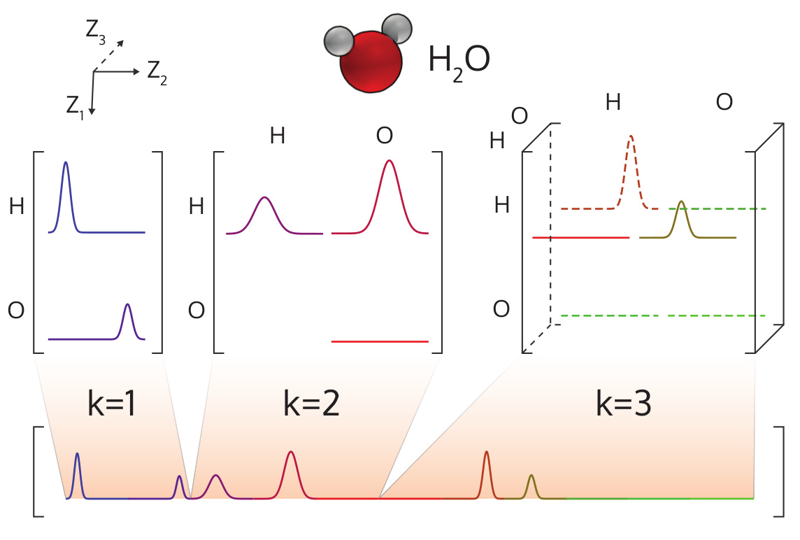
MBTR#

The many-body tensor representation (MBTR) encodes a structure by using a distribution of different structural motifs. It can be used directly for both finite and periodic systems. MBTR is especially suitable for applications where interpretability of the input is important because the features can be easily visualized and they correspond to specific structural properties of the system (distances, angles, dihedrals).

The MBTR representation can be used as a global representation (one feature vector per system) or as an atom-centered or local one (one feature vector per atom). As a global descriptor, the individual contributions are discretised on a single spectrum for the molecule as shown in the below figure.

bla

import collections.abc
collections.Iterable = collections.abc.Iterable # this is unfortunately necessary for compatbility of describe with Py>=3.10
from dscribe.descriptors import MBTR

min_dist = 0.8  #smallest distance in Angstrom
max_dist = 12.0  #largest distance in Angstrom
#we are constructing MBTR with inverse distances
grid_min = 1.0/max_dist # 1/Angstrom
grid_max = 1.0/min_dist # 1/Angstrom
grid_n = 100 # number of grid points
sigma = 0.05

#k=1, 1-body
#"atomic_number": The atomic number.
#k=2, 2-body
#"distance": Pairwise distance in angstroms.
#"inverse_distance": Pairwise inverse distance in 1/angstrom.
#k=3, 3-body
#"angle": Angle in degrees.
#"cosine": Cosine of the angle.

# MBTR setup for cyclohexane dataset
mbtr = MBTR(
    species=["H", "C"],
    geometry={"function": "inverse_distance"}, # only 2-body terms, no 3-body
    grid={"min": grid_min, "max": grid_max, "n": grid_n, "sigma": sigma},
    weighting={"function": "exp", "scale": 0.5, "threshold": 1e-3},
    periodic=False,
    normalization="l2",
    sparse=False
)

mbtrs = mbtr.create(traj)
#mbtrs = mbtr.create(traj[:10])
print(mbtrs.shape)

plt.plot(mbtrs[0])
plt.title('Full MBTR vector for one molecule')


# Create the mapping between an index in the output and the corresponding
# chemical symbol
n_elements = len(mbtr.species)
x = np.linspace(grid_min, grid_max, grid_n)

# Plot k=2
if mbtr.k==2:
    fig, ax = plt.subplots()
    for i in range(n_elements):
        for j in range(n_elements):
            if j >= i:
                i_species = mbtr.species[i]
                j_species = mbtr.species[j]
                loc = mbtr.get_location((i_species, j_species))
                plt.plot(x, mbtrs[0][loc], label="{}-{}".format(i_species, j_species))
    if mbtr.geometry['function'] == 'inverse_distance':
        ax.set_xlabel("Inverse distance (1/angstrom)")
    else:
        ax.set_xlabel("distance (angstrom)")
    plt.title('Individual components')

#plot k=3
if mbtr.k==3:
    fig, ax = plt.subplots()
    for i in range(n_elements):
        for j in range(n_elements):
            for k in range(n_elements):
                        i_species = mbtr.species[i]
                        j_species = mbtr.species[j]
                        k_species = mbtr.species[k]
                        loc = mbtr.get_location((i_species, j_species, k_species))
                        plt.plot(x, mbtrs[0][loc], label="{}-{}-{}".format(i_species, j_species, k_species))
    if mbtr.geometry['function'] == 'angle':
        ax.set_xlabel("angle in rad")
    else:
        ax.set_xlabel("cos(angle)")

    plt.title('Individual components')


ax.legend()
plt.show()

Task for you

Can you explain why the MBTR descriptor has the length it does?
Is this the optimal distance range to be considered? What does the value of sigma do to the descriptor?
What impact does it have to use 1-body, 2-body, 3-body components? How large is the descriptor in each case?
Play around with MBTR parameters a bit to find the optimal settings, then revert to the original settings provided.
Does MBTR satisfy all our symmetry requirements?

(Hint: pick a small set of geometries traj[0:10] to play around with settings to reduce computing time)

Task for you

Set up an MBTR feature representation for the QM7 dataset and play around with the parameters (Make sure to give the MBTR object a different name, e.g. mbtr_qm7)

# space to play around

SOAP#

Smooth Overlap of Atomic Positions (SOAP) is a descriptor that encodes atomic environments by using a local expansion of a gaussian smeared atomic density with orthonormal functions based on spherical harmonics and radial basis functions.

\[ p^{Z_1 Z_2}_{n n' l} = \pi \sqrt{\frac{8}{2l+1}}\sum_m {c^{Z_1}_{n l m}}^*c^{Z_2}_{n' l m} \]

here $n$ and $n'$ are indices for the different radial basis functions up to $n_\mathrm{max}$, $l$ is the angular degree of the spherical harmonics up to $l_\mathrm{max}$ and $Z_1$ and $Z_2$ are atomic species.

The coefficients $c^Z_{nlm}$ are defined as the following inner products:

\[ c^Z_{nlm} =\iiint_{\mathcal{R}^3}\mathrm{d}V g_{n}(r)Y_{lm}(\theta, \phi)\rho^Z(\mathbf{r}). \]

where $\rho^Z(\mathbf{r})$ is the gaussian smoothed atomic density for atoms with atomic number $Z$ defined as

\[ \rho^Z(\mathbf{r}) = \sum_i^{\lvert Z_i \rvert} e^{-1/2\sigma^2 \lvert \mathbf{r} - \mathbf{R}_i \rvert^2} \]

$Y_{lm}(\theta, \phi)$ are the real spherical harmonics, and $g_{n}(r)$ is the radial basis function.

For the radial degree of freedom, $g_{n}(r)$, multiple approaches may be used. By default the DScribe implementation uses spherical gaussian type orbitals as radial basis functions, as they allow faster analytic computation.

The SOAP similarity kernel between two atomic environments can be retrieved as a normalized polynomial kernel of the partial power spectrums: $$ K^\mathrm{SOAP}(\mathbf{p}, \mathbf{p'}) = \left( \frac{\mathbf{p} \cdot \mathbf{p'}}{\sqrt{\mathbf{p} \cdot \mathbf{p}~\mathbf{p'} \cdot \mathbf{p'}}}\right)^{\xi} $$

Starting point for parameters:

r_cut=3.5: we are considering 3.5A radius of sphere for describing each atom environments. For cyclohexane, this includes the whole ring, which is necessary to differentiate conformers. For QM7, this will likely be quite different.
n_max=4: expand over 4 radial GTO bases
l_max=4: expand over the first 4 spherical harmonics
sigma=0.3: assume each atom has a gaussian of width sigma=0.3 imposed on its lattice site

SOAP is a descriptor centred around atoms. For the construction of machine learning interatomic potentials, this is beneficial.

import collections.abc
collections.Iterable = collections.abc.Iterable # this is unfortunately necessary for compatbility of describe with Py>=3.10
from dscribe.descriptors import SOAP

species = ["H", "C"]
r_cut = 3.5 #cutoff in Angstrom
n_max = 4 # 
sigma = 0.3 #stdev of gaussians
l_max = 4

# Setting up the SOAP descriptor
soap = SOAP(
    species=species,
    periodic=False,
    r_cut=r_cut,
    n_max=n_max,
    l_max=l_max,
    sigma=sigma,
)

# Create SOAP output for all frames
soaps = soap.create(traj[:10])
#soaps = soap.create(traj)
print(soaps.shape)

We get a descriptor array with 3 dimensions: no. of frames, no. of atoms, and length of SOAP feature vector.

This is the input we need to fit machine learning interatomic potentials.

plt.plot(soaps[0,0,:]) #plot the soap vector for the first geometry, first atom
plt.title('Full SOAP feature vector for 1st geometry, 1st atom')

Task for you

Play around with r_cut, n_max, l_max and study how the length of the descriptor changes.
Show that the SOAP descriptors are also invariant w.r.t. to translations, permutations, and rotations

# space to play around

Measuring the similarity of structures becomes easy when the feature vectors represent the whole structure, such as in the case of Coulomb matrix or MBTR. In these cases the similarity between two structures is directly comparable with different kernels, e.g. the linear or Gaussian kernel.

Sometimes, we are focussed on comparative analysis between systems, then it is more useful to have a global descriptor. We can transform SOAP (and other atom-centered descriptors) into a global descriptor. We can achieve this by generating an average kernel. DScribe enables this with the option average='inner'.

# Setting up the SOAP descriptor
soap = SOAP(
    species=species,
    periodic=False,
    r_cut=r_cut,
    n_max=n_max,
    l_max=l_max,
    sigma=sigma,
    average='inner',
)

# Create SOAP output for all frames
soaps = soap.create(traj[:10])
#soaps = soap.create(traj)
print(soaps.shape)

Now we get only one SOAP descriptor per frame as we have averaged over the atoms

plt.plot(soaps[0,:]) #plot the soap vector for the first geometry, first atom
plt.title('Full SOAP feature vector for 1st geometry, 1st atom')

counts, bins = np.histogram(soaps.flatten(),bins=100)
#plt.stairs(counts, bins)
plt.hist(bins[:-1], bins, weights=counts)
plt.xlabel('SOAPS')
plt.ylabel('count')
plt.show()

Tasks for you

When SOAP is an atom-centered descriptor, 3.5 Angstrom cutoff radius around each atom pretty much covers all relevant information for cyclohexane. When we average and create a global descriptor, is this still the case?
Try to generate SOAP descriptors for the QM7 dataset. We will need this later.

#space to play around

We will now generate several different SOAP descriptors for the cyclohexane dataset (probably a good time to stretch your legs, grab a drink or take a break)

#Let's generate two different soap descriptors with different settings so we hvae them handy
import collections.abc
collections.Iterable = collections.abc.Iterable # this is unfortunately necessary for compatbility of describe with Py>=3.10
from dscribe.descriptors import SOAP

####DEFAULT SOAP

species = ["H", "C"]
r_cut = 3.5 #cutoff in Angstrom
n_max = 4 # 
sigma = 0.3 #stdev of gaussians
l_max = 4

# Setting up the SOAP descriptor
soap = SOAP(
    species=species,
    periodic=False,
    r_cut=r_cut,
    n_max=n_max,
    l_max=l_max,
    sigma=sigma,
    average='inner',
)

soaps_default = soap.create(traj)

####SOAP with high n and l

species = ["H", "C"]
r_cut = 3.5 #cutoff in Angstrom
n_max = 6 # 
sigma = 0.3 #stdev of gaussians
l_max = 6

# Setting up the SOAP descriptor
soap = SOAP(
    species=species,
    periodic=False,
    r_cut=r_cut,
    n_max=n_max,
    l_max=l_max,
    sigma=sigma,
    average='inner',
)

soaps_high = soap.create(traj)

#### SOAP with even higher n and l and larger cutoff

#soap_big = SOAP(
#    species=species,
#    periodic=False,
#    r_cut=4.0,
#    n_max=8,
#    l_max=6,
#    sigma=0.3,
#    average='inner',
#)

#soaps_big=soap.create(traj)#, n_jobs=6) # we can parallelize over cores with n_jobs to speed things up

Tasks for you

Which of the three descriptors with default parameters is likely to be the best? Rank them by their computational expense for the ML tasks that follow below?
Before moving on, please go back to CM and MBTR and make sure you reset all values to default and generate descriptors for the full cyclohexane dataset and the QM7 dataset.

Part 3: Similarity Analysis#

We can use our new descriptors to find the configurational change of the planar configuration without knowing anything about the structure. In the following box, we use a pairwise kernel from scikit-learn to compare structures for their similarity. For each trajectory, we compare the last frame with all other frames. We have the CM, the MBTR (inverse distance), and the three SOAP vectors to compare initially. Of course, you can play around with settings of all descriptors to find even better representations.

The ability of a descriptor to measure “distances” in the space of the dataset is a crucial prerequisite for being able to build reliable machine learning models.

#descriptors = soaps_default
#descriptors = soaps_high
#descriptors = coulomb_matrices
descriptors = mbtrs

#descriptors = soaps_big

similarities = np.zeros((len(traj), 5))
kernel = partial(pairwise_kernels, metric='rbf', gamma=2.0) #allows us to call pairwise_kernel like a function later

ranges2 = ranges.copy()
ranges2[4,1] = -1
for i, ci in enumerate(tqdm(conf_idx)):
    ki = kernel(descriptors[ranges2[i,0]].reshape(1,-1), descriptors)
    similarities[:, i] = ki

fig, ax = plt.subplots(1, figsize=(3*4.8528, 3*1.2219))

for i, (n, c, r, rgb) in enumerate(zip(names, c_energy, ranges, rgb_colors)):
    ax.plot(range(0, r[1] - r[0]),
            similarities[r[0]:r[1],i],
            label=n,
            c=rgb,
            zorder=-1)
    
ax.legend()
ax.set_xlabel("Simulation Timestep")
ax.set_ylabel("Similarity")

ax.set_xlim([0, len(energy)//5])
#ax.set_ylim([-0.1, 1.25 * (max_e - min_e)])
#ax.set_yticklabels([])

plt.tight_layout()
plt.savefig('similarity_soap_big.png')
plt.show()

A low similarity means that the descriptor considers the structures to be maximally unsimilar.

As we can see, the coulomb matrix is not good at identifying similarity. (See what happens with ‘sorted_l2’ and ‘eigenspectrum’. What is the origin of the difference?)
MBTR and SOAP do a lot better.
Using the SOAP descriptors, we see that all configurations retain similarity with the initial structure during the dynamics except for the planar structure, which starts in a structure that is disimilar to the final frame.

Task for you

Go back up and retry this with the CM and MBTR descriptors with different settings. Then try tuning the SOAP with higher n_max and l_max. Can you improve the similarity description with MBTR and SOAP? Which descriptor performs best? The similarity difference between the initial and final structure of the planar geometry is a good indicator of the “resolving power” of the descriptor. Before we do any machine learning, we should make sure that the resolving power and the structural covariance that our descriptor captures is as large as possible. The descriptor that achieves the biggest disimilarity between different structures should be our descriptor of choice.

#space to play

Task for you

If time permits, try to do the same for the QM7 dataset. Just look at the similarity between two molecules. Which descriptor best captures (dis)similarity between structures?

#space to play

Part 4: Dimensionality Reduction#

Let’s look at dimensionality reduction and clustering techniques. Can we come up with representations that clearly resolve the structural differences in the data?

Principal Component Analysis (PCA)#

PCA is the simplest linear dimensionality reduction technique based on Singular value Decomposition. The idea is to find a small set of principal components that represent the maximum amount of variance (diversity) in the data. We then project the data into that lower dimensional space. There are many variations on this technique including non-linear ones (Kernel PCA).

from sklearn.decomposition import PCA

#pick either 
descriptors = soaps_default
#descriptors = soaps_high
#descriptors = soaps_big
#descriptors = coulomb_matrices
#descriptors = mbtrs

n_components = 5

pca = PCA(n_components=n_components) #looking at the 5 largest eigenvalues
pca.fit(descriptors)
print(pca.explained_variance_ratio_)
print(pca.singular_values_)
# this is the part where we transform the data into the PCA representation. Now each element of the descriptor corresponds to the respective PCA eigenvalue
X_new = pca.transform(descriptors) 

plt.xlabel("PCA components")
plt.ylabel("Variance ratio")

plt.bar(np.arange(5),pca.explained_variance_ratio_, edgecolor='black')

print('Total variance of {0} lowest eigenvalues: {1}'.format(n_components, np.sum(pca.explained_variance_ratio_)))
print('Total variance of 2 lowest eigenvalues {0}'.format(np.sum(pca.explained_variance_ratio_[:2])))

The above plot shows us the variance captured by the 5 largest eigenvalues. Together the 5 components dominantly represent the data. The 2 lowest components cover a significant part of the variance.

Task for you

Which descriptor gives the highest variance for the first two PCA components? Can you tune that descriptor to maximize that number?

We pick the two components with the highest variance over the data and plot them against each other

print(X_new.shape)
descriptors = X_new[:,:2]
print(descriptors.shape)

fig, ax = plt.subplots(1, 1)

for (r, rgb) in zip(ranges,rgb_colors):
    ax.scatter(descriptors[r[0]:r[1],0], descriptors[r[0]:r[1],1], edgecolors='white', color=rgb, linewidths=0.4, label="datapoints", alpha=0.8)

plt.xlabel("PC1")
plt.ylabel("PC2")
fig.set_figheight(6.0)
fig.set_figwidth(6.0)

plt.show()

Let’s only plot the ‘planar’ trajectory and colour the dots according to the trajectory time. Red are early times, blue are late times.

fig, ax = plt.subplots(1, 1)

cm = plt.get_cmap('RdYlBu')
colors = range(10000)

sc = ax.scatter(descriptors[40000:,0], descriptors[40000:,1], edgecolors='white', 
            c=colors, linewidths=0.4, label="datapoints", alpha=0.8, cmap=cm)
fig.colorbar(sc)


plt.xlabel("PC1")
plt.ylabel("PC2")
fig.set_figheight(6.0)
fig.set_figwidth(6.0)

plt.show()

We can see that the deformation of the molecule out of the planar geometry can be captured well with the two principal components. However, the subtle differences between structures are not well resolved. We will try another method below.

Task for you

Compare the PCA plots for CM, MBTR, SOAP(n_max=4, l_max=4) (soaps_default), SOAP(n_max=6,l_max=6) (soaps_high).

t-SNE#

t-Distributed Stochastic Neighbor Embedding (t-SNE) is a popular dimensionality-reduction algorithm for visualizing high-dimensional data sets. It can be very informative (and sometimes also a bit misleading). Both methods are nonlinear (in contrast to PCA). t-SNE focuses on preserving the pairwise similarities between data points in a lower-dimensional space. t-SNE is concerned with preserving small pairwise distances whereas, PCA focuses on maintaining large pairwise distances to maximize variance.

So PCA preserves the variance in the data, whereas t-SNE preserves the relationships between data points in a lower-dimensional space, making it quite a good algorithm for visualizing complex high-dimensional data and relationships between individual datapoints.

Popular libraries for t-SNE (or an alternative algorithm called UMAP) are

from openTSNE import TSNE

#list of colors where each point is colored according to its trajectory

subsampling = 10 #consider only every 10th datapoint

data_length = 10000//subsampling

colors = []
for c in rgb_colors:
    for i in range(data_length):
        colors.append(c)

#list of colors for one trajectory which indicates time


##pick a descriptor
descriptors = soaps_default[::subsampling,:]
#descriptors = soaps_high[::subsampling,:]
#descriptors = soaps_big[::subsampling,:]
#descriptors = coulomb_matrices[::subsampling,:] 
#descriptors = mbtrs[::subsampling,:]

The perplexity is an important tunable parameter for t-SNE. Here we can see how increasing the perplexity (number of expected neighbors) changes the layout of the projection.

This algorithm may take several minutes. Be sure to parallelize it (n_jobs) and be patient. Above, we have already sliced the datasets to only take every 10th datapoint (1000 data points for each trajectory).

perplexities = np.logspace(0, 2.69, 6, dtype=int)
fig, ax = plt.subplots(1,
                       len(perplexities),
                       figsize=(4 * len(perplexities), 4),
                      )

for i, perp in enumerate(tqdm(perplexities)):
    tsne = TSNE(
        n_components=2,  # number of components to project across
        perplexity= perp, 
        metric="euclidean",  # distance metric
        n_jobs=6,  # parallelization
        random_state=42,
        verbose=False,
    )
    t_tsne = tsne.fit(descriptors)
    ax[i].scatter(*t_tsne.T, c=colors, s=2)
    ax[i].axis('off')
    ax[i].set_title("Perplexity = {}".format(perp))
plt.show()

For MBTR and SOAP and for large enough perplexity values, we find that the data clusters into 2 very large clusters and 1 very little one. The colours we are using are still the colours associated with the five cyclohexane MD runs. The t-SNE is proof that the 5 conformers start in different places but equilibrate into only two structures, namely the boat (green, red, yellow trajectories) and the chair conformation (blue and purple trajectories).

Now let’s take the most suitable perplexity value and look at the t-SNE, but now we color it according to the trajectory time. Red points are early, purple points are towards the end of the trajectory. We represent the different trajectory types with different markers. FOcus on the circles (planar trajectory).

perplexity = 50
plt.figure(figsize=(4,4),dpi=300)

cm = plt.cm.get_cmap('RdYlBu')
colors_time = []
for r in range(5):
    for i in np.linspace(0,1,data_length):
        colors_time.append(cm(i))

markers = []
for c in ['v','^','<','>','o']:
    for i in range(data_length):
        markers.append(c)

tsne = TSNE(
    n_components=2,  # number of components to project across
    perplexity=perplexity,  # amount of neighbors one point is posited to have... play around with this!
    metric="euclidean",  # distance metric
    n_jobs=4,  # parallelization
    random_state=42,
    verbose=False,
)

size = 4
t_tsne = tsne.fit(descriptors)
for i,m in enumerate(['v','^','<','>','o']):
    r = ranges[i]//subsampling
    tmp = t_tsne[r[0]:r[1]]
    plt.scatter(*tmp.T, c=colors_time[r[0]:r[1]], marker=m, s=size)

plt.axis('off')
plt.title("Perplexity = {}".format(perplexity))
plt.show()

The planar trajectory (circles) starts off in a place that is structurally similar to the initial configurations of the boat (yellow previousy, ‘>’ signs here) trajectory. While the boat trajectory converges into the same space as the half-chair and twist-boat, the planar trajectory moves through the half-chair configuration and the boat configuration before it ends up in the chair configuration.

Task for you:

A big part of ML and data science is data visualization. Can you come up with a better way to visualize the dynamical changes of conformations along the trajectories based on what we know now?

#space to play around

Task for you:

Surely, now you might be interested to make PCA plots of QM7. Can you plot the molecules into a 2D PCA descriptor space?

#space to play around

Part 5: Clustering#

Let’s assume we use PCA or t-SNE to perform dimensionality reduction and in the process, we have found a way to visualize the landscape of the data and relevant similarities. If we trust the space, we might want to perform clustering to identify the $n$ most structurally diverse geometries from this space.

This would allow us for example to pick a set of structures that best represent the diversity of this space to perform subsequent electronic structure calculations.

We will use k-means clustering based on the previous PCA to achieve this. We will use the computationally more efficient batched variant of KMeans.

from sklearn.decomposition import PCA

#pick either 
descriptors = soaps_default
descriptors = soaps_high
#descriptors = soaps_big
#descriptors = coulomb_matrices
#descriptors = mbtrs

###regenerate PCA
n_components = 5
pca = PCA(n_components=n_components)
pca.fit(descriptors)
X_new = pca.transform(descriptors) 
print(X_new.shape)
descriptors = X_new[:,:2]

from sklearn.cluster import MiniBatchKMeans

niter = 1000000
minibatch = 1800 # Batch size (how many data points are treated in the algorithm at once, reduce if you run out of memory)
ncluster= 20 # number of clusters

kmeans = MiniBatchKMeans(n_clusters=ncluster,
                        init="k-means++",
                        max_iter=niter,
                        n_init=3,
                        batch_size=minibatch)
# Fit the clustering model
km = kmeans.fit(np.array(descriptors).reshape(-1,1))
# Use the clustering model to predict the cluster number of each data point
indices = km.fit_predict(descriptors)

Once we have performed the clustering, we can calculate the centres of clusters, that is, the indices of the datapoints that are closest to the centroids of the clusters.

from sklearn.metrics.pairwise import pairwise_distances_argmin

centroid = kmeans.cluster_centers_
b = np.inf
ind = pairwise_distances_argmin(centroid, descriptors) # measure which structure is closest to the centroids of the clusters
print(ind)

X_centers = []
for i in ind:
    X_centers.append(descriptors[i])
X_centers = np.array(X_centers)

Now you could save the indices and you can identify which conformations belong to thse clusters. Let’s look at them

mol_traj = []
for i in ind:
    mol_traj.append(traj[i])

# visualize the trajectory of the clustered molecules
viewer = WeasWidget()
viewer.from_ase(mol_traj)
viewer.avr.model_style = 1
viewer.avr.show_hydrogen_bonds = True
viewer

Now we replot the PCA plot while coloring the different clusters and highlighting their centres.

fig, ax = plt.subplots(1, 1)

ax.scatter(X_new[:,0], X_new[:,1],c=indices, edgecolors='white', linewidths=0.4, label="datapoints", alpha=0.8)
ax.scatter(X_centers[:,0],X_centers[:,1],color="white",label="centers",edgecolors='black',linewidths=0.7,marker="X", alpha=0.8)

plt.legend(fancybox=True,framealpha=1,edgecolor='black',handletextpad=0.05,borderpad=0.3,handlelength=1.2,columnspacing=0.4,labelspacing=0.2,ncol=1,loc=1, fontsize="medium") #, bbox_to_anchor=(1.75, 1.02))
plt.xlabel("PC1")
plt.ylabel("PC2")
fig.set_figheight(6.0)
fig.set_figwidth(6.0)

plt.show()
# Two distinct parts of PC1/2 space, so pick enough clusters to avoid clusters spanning both parts. 

We can also see if our clusters cover a wide range of values for PC1

from matplotlib.ticker import MaxNLocator, FuncFormatter

ax = plt.axes()

ax.scatter(X_new[:,0], indices, edgecolors='white', linewidths=0.4, alpha=0.8)

plt.xlabel("PC1")
plt.ylabel("Cluster")
ax.xaxis.set_major_locator(MaxNLocator(integer=True))
ax.yaxis.set_major_locator(MaxNLocator(integer=True))

plt.show()

Task for you:

Try playing around with the number of clusters. How big a number would still be a sensible set of clusters?

This is a very simplified example of clustering and if the PCA and the descriptors are not resolving the diversity of the space really well, you are running the risk of selecting “diverse” structures with the wrong measure. There are many more advanced methods for clustering, which you should explore. I recommend the resource on Unsupervised Learning quoted at the top of the notebook and the links at the end of the notebook.

Part 6: Supervised Learning / Model Fitting#

In a later tutorial, you will learn all about neural networks and deep learning models for interatomic potentials. Here, we will look at models based on linear regression and Kernel Ridge Regression as they form a good starting point. Our aim is to create a model that can predict the energy of any cyclohexane conformation. The previously calculated feature vectors (descriptors) are our input quantities ($\mathbf{x}$), the energies are our labels.

#pick either 
#descriptors = soaps_default
descriptors = soaps_high
#descriptors = soaps_big
#descriptors = coulomb_matrices
#descriptors = mbtrs

Data Preparation#

First we have to split our data into train and test data. The train data is what we will use to train the model. The test data will be “unseen” and used to evaluate the prediction capabilities of the model.

We won’t be training on the full training data set, but only on a small subset. We will take 1000 data points.

from sklearn.model_selection import train_test_split
from sklearn.utils import resample

#we know the `energy`` of each frame, the energy of the starting conformers (c_energy), max_e, and min_e

X = descriptors
#our labels are the energies
y = energy

X_train_full, X_test, y_train_full, y_test = train_test_split(
    X, y, #inputs and outputs
    test_size=0.20, #20% of the data is test data
    random_state=42, #a random seed
    ) 

#only train on a small subset of samples rather than the full training dataset
X_train, y_train = resample(X_train_full, y_train_full, replace=False, n_samples=1000, random_state=42)

Next, we standardize the training and testing sets. This means scaling and normalizing the data. This way, the model mean is centred around zero and the model does not have to cover large value ranges. We do this with the inputs and the outputs.

For the labels/outputs, this is as simple as $$ \tilde{\mathbf{y}} = \frac{\mathbf{y} - u}{s} $$ where u and s are the mean and the standard deviation of the labels.

from sklearn import preprocessing

#scikit-learn has a utility to help with the feature vectors

scaler = preprocessing.StandardScaler()
scaler.fit(X_train)
X_train = scaler.transform(X_train)
X_test = scaler.transform(X_test) #? This needs to be the same scaler as for the training data, otherwise the test data would be scaled into the wrong space

#rescaling the labels

u = np.mean(y_train)
s = np.std(y_train)

y_train_scaled = (y_train-u)/s
y_test_scaled = (y_test-u)/s

def unscale(y):
    # this is for transforming the predictions back into proper energies
    return (y*s)+u

Multiple Linear Regression#

In multiple linear regression, we try to find a set of regression coefficients $\mathbf{\beta}$ to approximate a $p$-dimensional function

\[ f(\mathbf{x};\mathbf{\beta}) = \sum_{j=1}^{p} \beta_j x_j = \mathbf{x}^T \mathbf{\beta} \]

In our case, we would like to predict the energy for an arbitrary conformation of cyclohexane. We have already acknowledged that this would not be possible based simply on the Cartesian positions of atoms, which is why we have created various representations that provide us with high dimensional feature vectors (e.g. SOAP).

The feature vectors form the inputs $\mathbf{x}$ and the dimensionality of the space ($p$) in which we want to fit a linear relationship is the length of the descriptor. The quality of the fit will depend on the ability of the high dimensional space spanned by the descriptor to express complex relationships as linear trends. The more chemically meaningful (and higher dimensional) the descriptor, the better the fit.

Let’s test this for the energy prediction.

from sklearn.linear_model import LinearRegression

multiple_linear_regression = LinearRegression()
multiple_linear_regression.fit(X = X_train, y = y_train_scaled)
# This is the training part

Determine $R^2$, MAE, and RMSD of the fit

$R^2$ metric (Coefficient of determination) $$ R^2 = 1 - \frac{\sum_i(y_i-f_i)^2}{\sum_i(y_i-u)^2} $$ where $u$ is the mean of the observed data, $y_i$ is the data value ("ground truth") and $f_i$ is the prediction.

Mean Absolute Error (MAE) $$ \mathrm{MAE} = \frac{\sum_i |y_i - f_i|}{n} $$

Root Mean Square Error (RMSE) $$ \mathrm{RMSE} = \sqrt{\frac{\sum_{i} (y_i - f_i)^2}{n} } $$

# This is the prediction part
from sklearn.metrics import r2_score, mean_squared_error, mean_absolute_error

pred_train_lr = unscale(multiple_linear_regression.predict(X_train))
pred_test_lr = unscale(multiple_linear_regression.predict(X_test))

r2 = r2_score(y_test, pred_test_lr)
print('R2 train = ', r2_score(y_train, pred_train_lr))
print('R2 test = ', r2_score(y_test, pred_test_lr))

mae = mean_absolute_error(y_test, pred_test_lr)
print('MAE test = ', mae)
rmse = np.sqrt(mean_squared_error(y_test,pred_test_lr ))
print('RSME test = ', rmse)

plt.scatter(y_train,pred_train_lr, label='Training Set')
plt.scatter(y_test,pred_test_lr, label='Test Set')

plt.xlabel('Real')
plt.ylabel('Predicted')
plt.legend()

Task for you

Which of the descriptors that we have prepared gives the best correlation and test error with a simple linear fit?
What value of MAE or RMSE on the test set should we consider to be a low error? What are the energy differences between conformers that we need to be able to resolve?

Kernel Ridge Regression (KRR) and Gaussian Process Regression (GPR)#

Kernel Ridge Regression provides a rigorous mathematical framework to extend linear statistical learning techniques to model nonlinear dependencies in high-dimensional data. The method is based on measuring similarity betwen pairs of data points and then using this similarity to unfold nonlinearities in the original data space. The similarity transformation enables the mapping of the data into a higher dimensional space spanned by the training data where the data might be representable in terms of linear functions.

If we start from linear regression $$ f(\mathbf{x};\mathbf{\beta}) = \sum_{j=1}^{p} \beta_j x_j = \mathbf{x}^T \mathbf{\beta} $$ we can expand the regression coefficients $\beta$ via different regression coefficients $\alpha$ in a much higher dimensional space spanned by the size of the training data ($N_{tr}$). $$ \beta_j = \sum_{i=1}^{N_{\mathrm{tr}}} \alpha_i x_{ij} $x_{ij}$ are elements of the input vectors (feature vectors based on our descriptors). By inserting into the above we get $$ f(\mathbf{x}') = \sum_{i=1}^{N_{tr}} \alpha_i \braket{\mathbf{x}_i,\mathbf{x}'} $$ where $\braket{\mathbf{x}_i,\mathbf{x}’}$ is a dot-product of two feature vectors, one associated with data point $i$ and the other one associated with the point for which we would like to make a prediction ($\mathbf{x}’$). The same can be written in some choice of nonlinearly transformed feature space: $$ f(\phi(\mathbf{x}')) = \sum_{i=1}^{N_{tr}} \alpha_i k(\mathbf{x}_i,\mathbf{x}') $$ where $k(\mathbf{x}_i,\mathbf{x}’)$ is the dot product in feature space (the so-called kernel). The kernel is the similarity measure with which we compare training datapoint $\mathbf{x}_i$ and the point to be predicted $\mathbf{x}’$.

If $k(\mathbf{x}_i,\mathbf{x}') = \braket{\mathbf{x}_i,\mathbf{x}'}$, it is called a linear kernel or dot-product kernel. This would be equivalent to linear regression.

We can also choose a Gaussian kernel: $$ k(\mathbf{x}_i,\mathbf{x}') = \exp \left(-\frac{1}{2\sigma^2}\sum_j^{p} (x_{ij} - x_j^{'})^2 \right) $$ This is equivalent to mapping the input vector to a space spanned by Gaussian functions (with width $\sigma$) centred at the training data points.

The term Ridge Regression comes from the fact that a simple inversion of the equation $\mathbf{y}=\mathbf{K}\mathbf{\alpha}$ to determine $\mathbf{\alpha}$ is numerically unstable. This is often connected with individual parameters becoming extremely large. In Ridge regression, we use a regularized form of linear regression, where we minimize the L2 loss between prediction and training data under the constraint that the coefficients remain small (Tikhonov regularization). That means, instead of solving $$ \mathbf{\alpha} = \mathbf{K}^{-1}\mathbf{y} $$ we solve $$ \mathbf{\alpha} = (\mathbf{K}^{-1}+\lambda\mathbf{I})\mathbf{y} $$ where $\mathbf{I}$ is the identity matrix and $\lambda$ is a small nonnegative smoothing parameter (regularization parameter). Regularization is crucial to reduce the risk of overfitting.

Gaussian kernel fits are defined by two hyperparameters, $\sigma$ and $\lambda$. If $\sigma$ is too small (Gaussians might not overlap), the model might not generalize well, but if $\sigma$ is too large, the model will fail to learn from the data.

Typically, hyperparameters within the ML model need to be optimised to achieve optimal accuracy and generalisability.

Gaussian Process Regresssion is related to KRR as it generates fits to the same mathematical form of the regression function, but it does so with a Bayesian approach that automatically gives the model variance as a byproduct. Another byproduct is that it often can automatically find optimal hyperparameters (via the log-marginal likelihood).

Let’s start by reproducing the linear fit with a linear kernel

from sklearn.kernel_ridge import KernelRidge

krr = KernelRidge(alpha=0.00001, kernel='linear') # alpha here is lambda in the explanation above
krr.fit(X_train, y_train_scaled)

from sklearn.metrics import r2_score, mean_squared_error, mean_absolute_error

pred_train_kr =  unscale(krr.predict(X_train))
pred_test_kr = unscale(krr.predict(X_test))

r2 = r2_score(y_test, pred_test_kr)
print('R2 train = ', r2_score(y_train, pred_train_kr))
print('R2 test = ', r2_score(y_test, pred_test_kr))

mae = mean_absolute_error(y_test, pred_test_kr)
print('MAE test = ', mae)
rmse = np.sqrt(mean_squared_error(y_test,pred_test_kr ))
print('RSME test = ', rmse)

plt.scatter(y_train,pred_train_kr, label='Training Set')
plt.scatter(y_test,pred_test_kr, label='Test Set')

plt.xlabel('Real')
plt.ylabel('Predicted')
plt.legend()

Next we try the Gaussian (RBF) kernel. Here we have to set the width of the RBFs

from sklearn.kernel_ridge import KernelRidge

krr = KernelRidge(alpha=0.00001, kernel='rbf', gamma=0.005)
krr.fit(X_train, y_train_scaled)

from sklearn.metrics import r2_score, mean_squared_error, mean_absolute_error

pred_train_kr =  unscale(krr.predict(X_train))
pred_test_kr = unscale(krr.predict(X_test))

r2 = r2_score(y_test, pred_test_kr)
print('R2 train = ', r2_score(y_train, pred_train_kr))
print('R2 test = ', r2_score(y_test, pred_test_kr))

mae = mean_absolute_error(y_test, pred_test_kr)
print('MAE test = ', mae)
rmse = np.sqrt(mean_squared_error(y_test,pred_test_kr ))
print('RSME test = ', rmse)

plt.scatter(y_train,pred_train_kr, label='Training Set')
plt.scatter(y_test,pred_test_kr, label='Test Set')

plt.xlabel('Real')
plt.ylabel('Predicted')
plt.legend()

Note how the model fits the trained data almost perfectly and much better than the linear model, but does not capture the test data quite as well. This means we are overfitting. This can have several reasons:

The data is simple and the model is too complex
The feature space is too large
Too much noise and outliers in training data (can be excluded here)
Not enough data
The model is not sufficiently constrained and the hyperparameters are not optimal.

We need to find a way to properly evaluate and fine-tune the model.

In this case, the linear kernel is the right choice because the data is simple enough. There is no need to go to a Gaussian kernel, but we’ll still try to optimise what we can get out of the Gaussian kernel (for educational purposes).

Cross Validation#

Cross validation (CV) is a resampling method that uses different portions of data to test and train models. It is a way to assess how well a model generalises and to robustly evaluate model performance. We can also use cross validation to check for outliers in the dataset. As shown below, the data is split into training and test data. The test data is then further split into $k$ “folds” (here 5). Over $k$ possible permutations, we can change which part of the training data we “hold out”. That means we can train $k$ different models on different parts of the data. If the standard deviation over several folds is low, the model is robust. If the MAE on the hold-out set is very similar, it likely also has few outliers. The standard deviation can also provide us with a measure of the uncertainty of the model, which could be used in the context of committee-based active learning.

CV is also used when the space of hyperparameters is explored to find the optimal model layout. For KRR, this is $\sigma$ and $\lambda$, for neural networks, it can be parameters that define the layout of the network.

crossval

Let’s evaluate the mean prediction error and standard deviation for the linear model and the KRR model with given settings.

from sklearn.kernel_ridge import KernelRidge
from sklearn.model_selection import cross_validate
from sklearn.metrics import r2_score, mean_squared_error, mean_absolute_error, make_scorer

krr = KernelRidge(alpha=0.00001, kernel='linear')
#krr.fit(X_train, y_train_scaled) #? This would be fitting twice - Check documentation for the cross validation tool in question

#this is a dictionary which we can use to pass multiple scoring functions into CV (even custom-made ones)
scoring = {
    'r2_score': make_scorer(r2_score),
    'MAE': make_scorer(mean_absolute_error),
    'RMSE': make_scorer(mean_squared_error),
    }

scores = cross_validate(
    krr, #model
    X_train, #training data
    y_train_scaled, #training data
    scoring=scoring, # types of model scores
    cv=5, # k-foldedness of cross validation
    return_estimator=False, #this function can return all five models if needed
    return_train_score=True
    )

print('Linear Model')
print('Train Errors:')
print('    The mean and stdev of train MAE over the folds are {0:8.5f} and {1:8.5f} eV'.format(np.mean(scores['train_MAE']*s), np.std(np.sqrt(scores['train_MAE'])*s)))
print('    The mean and stdev of train RMSE over the folds are {0:8.5f} and {1:8.5f} eV'.format(np.mean(scores['train_RMSE']*s), np.std(np.sqrt(scores['train_RMSE'])*s)))
print('Test Errors:')
print('    The mean and stdev of test MAE over the folds are {0:8.5f} and {1:8.5f} eV'.format(np.mean(scores['test_MAE']*s), np.std(np.sqrt(scores['test_MAE'])*s)))
print('    The mean and stdev of test RMSE over the folds are {0:8.5f} and {1:8.5f} eV'.format(np.mean(scores['test_RMSE']*s), np.std(np.sqrt(scores['test_RMSE'])*s)))

from sklearn.model_selection import cross_validate
from sklearn.kernel_ridge import KernelRidge
from sklearn.metrics import r2_score, mean_squared_error, mean_absolute_error, make_scorer

krr = KernelRidge(alpha=0.00001, kernel='rbf', gamma=0.005)

#this is a dictionary which we can use to pass multiple scoring functions into CV (even custom-made ones)
scoring = {
    'r2_score': make_scorer(r2_score),
    'MAE': make_scorer(mean_absolute_error),
    'RMSE': make_scorer(mean_squared_error),
    }

scores = cross_validate(
    krr, 
    X_train, 
    y_train_scaled, 
    scoring=scoring, 
    cv=5, 
    return_estimator=False, #this function can return all five models if needed
    return_train_score=True
    )

print('RBF Model')
print('Train Errors:')
print('    The mean and stdev of train MAE over the folds are {0:8.5f} and {1:8.5f} eV'.format(np.mean(scores['train_MAE']*s), np.std(np.sqrt(scores['train_MAE'])*s)))
print('    The mean and stdev of train RMSE over the folds are {0:8.5f} and {1:8.5f} eV'.format(np.mean(scores['train_RMSE']*s), np.std(np.sqrt(scores['train_RMSE'])*s)))
print('Validation Errors:')
print('    The mean and stdev of test MAE over the folds are {0:8.5f} and {1:8.5f} eV'.format(np.mean(scores['test_MAE']*s), np.std(np.sqrt(scores['test_MAE'])*s)))
print('    The mean and stdev of test RMSE over the folds are {0:8.5f} and {1:8.5f} eV'.format(np.mean(scores['test_RMSE']*s), np.std(np.sqrt(scores['test_RMSE'])*s)))

Task for you

What have we learned and what do we have to do next? Which one of the listed causes of overfitting might be the case here?

Hyperparameter Optimisation#

We can use the CV to perform a systematic hyperparameter optimisation. In the following we use a scikit-learn feature to perform a hyperparameter grid search.

from sklearn.model_selection import cross_validate, GridSearchCV
from sklearn.kernel_ridge import KernelRidge
from sklearn.metrics import r2_score, mean_squared_error, mean_absolute_error, make_scorer
import pandas as pd

j = 0.000001
alphas = [ j*(10**i) for i in range(8)]
gammas = [ j*(10**(i/8)) for i in range(64)]

#vary alphas
#parameters = {'kernel':['rbf'], 'alpha':alphas, 'gamma':[0.005]}
#vary gammas
parameters = {'kernel':['rbf'], 'alpha':[0.0001], 'gamma':gammas}

scoring = {
    'r2_score': make_scorer(r2_score),
    'MAE': make_scorer(mean_absolute_error),
    'RMSE': make_scorer(mean_squared_error),
    }

krr = KernelRidge()
gridsearch = GridSearchCV(krr, 
param_grid=parameters, 
scoring=scoring, 
cv=5, 
n_jobs=6,
refit=False, 
return_train_score=True
)

gridsearch.fit(X_train, y_train_scaled)

cvdata = pd.DataFrame(gridsearch.cv_results_)

#try also printing the full dataframe by uncommenting the next line and commenting the other one out
#cvdata
cvdata[['param_alpha','param_gamma','param_kernel','mean_test_MAE', 'std_test_MAE', 'mean_train_MAE', 'std_train_MAE']]

cvdata['mean_test_MAE'] = cvdata['mean_test_MAE'].multiply(s) #unscale
cvdata['mean_train_MAE'] = cvdata['mean_train_MAE'].multiply(s) #unscale
#plotframe = cvdata[['param_alpha','mean_test_MAE','mean_train_MAE']]
#plotframe.plot('param_alpha')
plotframe = cvdata[['param_gamma','mean_test_MAE','mean_train_MAE']]
plotframe.plot('param_gamma',logx=True)


#? "train" should be "validation" again

We can exactly see at which RBF width value the train and test errors start to deviate. This is the point above which overfitting occurs. An alpha value of 0.0001 and a gamma value of 0.001 (RBF width) seem to provide improved results. Let’s use these to reevaluate the model and compare with the previous results.

from sklearn.model_selection import cross_validate
from sklearn.kernel_ridge import KernelRidge
from sklearn.metrics import r2_score, mean_squared_error, mean_absolute_error, make_scorer

krr = KernelRidge(alpha=0.0001, kernel='rbf', gamma=0.001)

#this is a dictionary which we can use to pass multiple scoring functions into CV (even custom-made ones)
scoring = {
    'r2_score': make_scorer(r2_score),
    'MAE': make_scorer(mean_absolute_error),
    'RMSE': make_scorer(mean_squared_error),
    }

scores = cross_validate(
    krr, 
    X_train, 
    y_train_scaled, 
    scoring=scoring, 
    cv=5, 
    return_estimator=False, #this function can return all five models if needed
    return_train_score=True
    )

print('Train Errors:')
print('    The mean and stdev of train MAE over the folds are {0:8.5f} and {1:8.5f} eV'.format(np.mean(scores['train_MAE']*s), np.std(np.sqrt(scores['train_MAE'])*s)))
print('    The mean and stdev of train RMSE over the folds are {0:8.5f} and {1:8.5f} eV'.format(np.mean(scores['train_RMSE']*s), np.std(np.sqrt(scores['train_RMSE'])*s)))
print('Test Errors:')
print('    The mean and stdev of test MAE over the folds are {0:8.5f} and {1:8.5f} eV'.format(np.mean(scores['test_MAE']*s), np.std(np.sqrt(scores['test_MAE'])*s)))
print('    The mean and stdev of test RMSE over the folds are {0:8.5f} and {1:8.5f} eV'.format(np.mean(scores['test_RMSE']*s), np.std(np.sqrt(scores['test_RMSE'])*s)))

Task for you

Use this grid search code as a starting point to identify the optimal parameters that will provide the lowest test error and will not lead to overfitting of the training data

Learning Curves#

Maybe we need more training data. Studying how quickly the prediction error goes down as we add training data means assessing the rate of learning of the model. Learning curves are important to undertsand the ability of models to learn from little data. We can use them to also compare across the four descriptors we have used.

Generating the learning curve data will take a little while.

Task for you

Study the plot below. Which descriptor achieves the highest error for the smallest training data set?

#only train on a small subset of samples rather than the full training dataset
from sklearn import preprocessing
from sklearn.utils import resample
from sklearn.kernel_ridge import KernelRidge
from sklearn.metrics import r2_score, mean_squared_error, mean_absolute_error
from sklearn.model_selection import cross_validate
from sklearn.kernel_ridge import KernelRidge
from sklearn.metrics import r2_score, mean_squared_error, mean_absolute_error, make_scorer

descriptors = [coulomb_matrices, mbtrs, soaps_default, soaps_high]
ndatas = [100, 500, 1000, 2500, 5500]

learning_curve = np.zeros([len(descriptors),len(ndatas),2])

for i,X in tqdm(enumerate(descriptors)):
    X_train_full, X_test, y_train_full, y_test = train_test_split(
        X, y, #inputs and outputs
        test_size=0.20, #20% of the data is test data
        random_state=42, #a random seed
    )
    for j,ndata in tqdm(enumerate(ndatas)):

        X_train, y_train = resample(X_train_full, y_train_full, replace=False, n_samples=ndata, random_state=42)
        scaler = preprocessing.StandardScaler()
        scaler.fit(X_train)
        X_train = scaler.transform(X_train)
        X_test = scaler.transform(X_test)

        #rescaling the labels
        u = np.mean(y_train)
        s = np.std(y_train)
        y_train_scaled = (y_train-u)/s
        y_test_scaled = (y_test-u)/s

        def unscale(y):
            # this is for transforming the predictions back into proper energies
            return (y*s)+u

        scoring = {
            'r2_score': make_scorer(r2_score),
            'MAE': make_scorer(mean_absolute_error),
            'RMSE': make_scorer(mean_squared_error),
        }

        krr = KernelRidge(alpha=0.0001, kernel='rbf', gamma=0.001)
        scores = cross_validate(
            krr, 
            X_train, 
            y_train_scaled, 
            scoring=scoring, 
            cv=5, 
            n_jobs=6,
            return_estimator=False,
            return_train_score=True
            )

        learning_curve[i,j,0] = np.mean(scores['test_MAE'])*s
        learning_curve[i,j,1] = np.std(scores['test_MAE'])*s

descriptor_names = ['CM', 'MBTR', 'SOAP_default', 'SOAP_high'] #, soaps_default, soaps_high]

for i, d in enumerate(descriptors):
    plt.errorbar(ndatas, learning_curve[i,:,0], learning_curve[i,:,1],label=descriptor_names[i])
plt.xlabel('number of training data points')
plt.ylabel('MAE in eV')
plt.legend()

Part 7: The Challenge#

Use the code above and your newly acquired skills to create a KRR model to predict the PBE0 atomization energy and the PBE0-DFTB3 delta energy of the QM7 dataset.

Try to use a tailored descriptor and a set of hyperparameters that provide you with the lowest possible MAE on the test set.

Use a 80%/20% train/test split with random_state=42 for reproducibility
You can use any of the descriptors that we have covered with any setting. The model just needs to feasibly train and predict in a reasonable timeframe.
Can you beat the MAE achieved in the original paper? (Phys. Rev. Lett. 108, 058301) ca. 10kcal/mol = 0.43 eV

Conclusion#

This is it. Hopefully, this gave a brief overview over some workflows and methods that are useful for ML applications in chemistry and materials research.

Where next for deeper insights into methods?

Check out the AI lectures and tutorials on the https://nomad-lab.eu/aitoolkitlist webpage Link: NOMAD AI Tutorials
“Quantum Chemistry in the Age of Machine Learning”, edited by Pavlo Dral (2022) with Github tutorials for each chapter
Work on your own project. The best way to learn is to work on a problem and to make mistakes!

Tutorial on Basics of Machine Learning in Computational Molecular Science

Contents

Tutorial on Basics of Machine Learning in Computational Molecular Science#

Prelude#

Part 1: Data Preparation and Analysis#

Read and analyse Molecular Dynamics Data#

Read and analyse QM7 molecule dataset#

Data Prep Summary#

Part 2: Generate Descriptors#

Coulomb Matrix#

MBTR#

SOAP#

Part 3: Similarity Analysis#

Part 4: Dimensionality Reduction#

Principal Component Analysis (PCA)#

t-SNE#

Part 5: Clustering#

Part 6: Supervised Learning / Model Fitting#

Data Preparation#

Multiple Linear Regression#

Kernel Ridge Regression (KRR) and Gaussian Process Regression (GPR)#

Cross Validation#

Hyperparameter Optimisation#

Learning Curves#

Part 7: The Challenge#

Conclusion#